Data management, wrangling, and best practices

Session details

Objectives

To learn the difference between “messy” and “tidy” data and see the advantages of using data that are consistently structured.
To perform simple data transformations and create summaries.
To get to know the tools that help tidying up and reshaping the data.

At the end of this session you will be able:

To write code using the %>% operator.
To perform simple data transformations using mutate().
To select variables and observations to work with using filter()and select().
To order data by variable using arrange().
To provide a simple data summary using group_by() and summarise().
To change the structure of the data using gather() (and optionally spread()).

Expected learning

For the final exercise of this session, you will try to get the data from the original data (using NHANES) to the table below. By using the code in this session, you will have acheived our learning expectations.

The final exercise will be to get this data:

NHANES

#> # A tibble: 10,000 x 76
#>       ID SurveyYr Gender   Age AgeDecade AgeMonths Race1 Race3 Education
#>    <int> <fct>    <fct>  <int> <fct>         <int> <fct> <fct> <fct>    
#>  1 51624 2009_10  male      34 " 30-39"        409 White <NA>  High Sch…
#>  2 51624 2009_10  male      34 " 30-39"        409 White <NA>  High Sch…
#>  3 51624 2009_10  male      34 " 30-39"        409 White <NA>  High Sch…
#>  4 51625 2009_10  male       4 " 0-9"           49 Other <NA>  <NA>     
#>  5 51630 2009_10  female    49 " 40-49"        596 White <NA>  Some Col…
#>  6 51638 2009_10  male       9 " 0-9"          115 White <NA>  <NA>     
#>  7 51646 2009_10  male       8 " 0-9"          101 White <NA>  <NA>     
#>  8 51647 2009_10  female    45 " 40-49"        541 White <NA>  College …
#>  9 51647 2009_10  female    45 " 40-49"        541 White <NA>  College …
#> 10 51647 2009_10  female    45 " 40-49"        541 White <NA>  College …
#> # … with 9,990 more rows, and 67 more variables: MaritalStatus <fct>,
#> #   HHIncome <fct>, HHIncomeMid <int>, Poverty <dbl>, HomeRooms <int>,
#> #   HomeOwn <fct>, Work <fct>, Weight <dbl>, Length <dbl>, HeadCirc <dbl>,
#> #   Height <dbl>, BMI <dbl>, BMICatUnder20yrs <fct>, BMI_WHO <fct>,
#> #   Pulse <int>, BPSysAve <int>, BPDiaAve <int>, BPSys1 <int>,
#> #   BPDia1 <int>, BPSys2 <int>, BPDia2 <int>, BPSys3 <int>, BPDia3 <int>,
#> #   Testosterone <dbl>, DirectChol <dbl>, TotChol <dbl>, UrineVol1 <int>,
#> #   UrineFlow1 <dbl>, UrineVol2 <int>, UrineFlow2 <dbl>, Diabetes <fct>,
#> #   DiabetesAge <int>, HealthGen <fct>, DaysPhysHlthBad <int>,
#> #   DaysMentHlthBad <int>, LittleInterest <fct>, Depressed <fct>,
#> #   nPregnancies <int>, nBabies <int>, Age1stBaby <int>,
#> #   SleepHrsNight <int>, SleepTrouble <fct>, PhysActive <fct>,
#> #   PhysActiveDays <int>, TVHrsDay <fct>, CompHrsDay <fct>,
#> #   TVHrsDayChild <int>, CompHrsDayChild <int>, Alcohol12PlusYr <fct>,
#> #   AlcoholDay <int>, AlcoholYear <int>, SmokeNow <fct>, Smoke100 <fct>,
#> #   Smoke100n <fct>, SmokeAge <int>, Marijuana <fct>, AgeFirstMarij <int>,
#> #   RegularMarij <fct>, AgeRegMarij <int>, HardDrugs <fct>, SexEver <fct>,
#> #   SexAge <int>, SexNumPartnLife <int>, SexNumPartYear <int>,
#> #   SameSex <fct>, SexOrientation <fct>, PregnantNow <fct>

To look like this:

Table 1: Mean values of characteristics for women and men between 18-75 years of age at each of the two survey years.
Gender	Measure	2009_10	2011_12
female	Age	44.02	44.15
female	AgeDiabetesDiagnosis	48.13	46.51
female	BMI	28.96	28.60
female	BPDiaAve	67.69	70.04
female	BPSysAve	116.04	117.90
female	DrinksOfAlcoholInDay	2.34	2.20
female	MoreThan5DaysActive	0.31	0.39
female	NumberOfBabies	2.44	2.31
female	Poverty	2.93	2.88
female	TotalCholesterol	5.14	5.11
male	Age	43.11	43.88
male	AgeDiabetesDiagnosis	47.58	45.14
male	BMI	28.76	28.70
male	BPDiaAve	70.94	73.14
male	BPSysAve	121.61	122.43
male	DrinksOfAlcoholInDay	3.52	3.71
male	MoreThan5DaysActive	0.29	0.36
male	NumberOfBabies	NaN	NaN
male	Poverty	3.01	2.97
male	TotalCholesterol	5.07	4.90

Managing and working with data in R

Recall that:

You should never edit your raw data (should be in data-raw/ folder)
Only work with your raw data using R code
Save the edited data as another dataset (should be in data/ folder)
Document and comment as best you can to help you remember
- But, let the code speak for itself (e.g. keep it simple, have intermediate and descriptive steps)

In data “wrangling”/“munging”/managing, most tasks can be broken down into only a few simple “verbs” (actions), as listed in the table.

Table 2: Data wrangling task, an example of the task, and the functions to use for data wrangling.
Tasks	Examples	Function
Choosing columns	Remove columns related to data entry, such as name of person entering data.	select()
Renaming columns	Changing a column name from 'Q1' to 'ParticipantName'.	rename()
Transforming or modifying columns	Multiplying a column's values; taking the log.	mutate()
Subsetting/filtering out rows/observations	Keeping rows with glucose values above 4.	filter()
Sorting/re-arranging rows	Show rows with the smallest value at the top.	arrange()
Converting from wide to long form	One row per participant to multiple participants per row (repeated measures).	gather()
Converting from long to wide form	Multiple rows per participant (repeated measures) to one participant per row.	spread()
Calculating summaries on the data	Calculating the maximum, median, and minimum age.	summarise()
Running analyses by group	Calculate means of age by males and females.	group_by() with summarise()

Wrangling here is used in the sense of maneuvering, managing, controlling, and turning your data around to better understand it and to prepare it for later analyses. The packages dplyr and tidyr provide easy tools for most common data manipulation tasks. For dplyr, it is built to work directly with data frames and has an additional feature to interact directly with data stored in an external database, such as in SQL. Working with databases is powerful as you can work with massive datasets (100s of GB), more than your computer could normally handle. This won’t be covered, but see this resources from Data Carpentry) to learn more.

A tip when doing complicated wrangling and you get the data to a form that you like and will use often: Save it as an “output” dataset in the data/ folder so you can easily use it again later rather than run the wrangling code everytime.

Loading the packages and dataset

We’re going to use the US NHANES dataset. There is an NHANES package that contains a teaching version of the original dataset, so we’ll use that for this lesson. First, make sure the R Project you created previously is open. Then open the R/wrangling-session.R script to start typing out the next code. We’ll use this file to write the code for this session (but not for the exercises).

# Load up the packages
# tidyverse contains the dplyr and tidyr packages
library(tidyverse)
library(NHANES)

# Briefly glimpse contents of dataset
glimpse(NHANES)

#> Observations: 10,000
#> Variables: 76
#> $ ID               <int> 51624, 51624, 51624, 51625, 51630, 51638, 51646…
#> $ SurveyYr         <fct> 2009_10, 2009_10, 2009_10, 2009_10, 2009_10, 20…
#> $ Gender           <fct> male, male, male, male, female, male, male, fem…
#> $ Age              <int> 34, 34, 34, 4, 49, 9, 8, 45, 45, 45, 66, 58, 54…
#> $ AgeDecade        <fct>  30-39,  30-39,  30-39,  0-9,  40-49,  0-9,  0-…
#> $ AgeMonths        <int> 409, 409, 409, 49, 596, 115, 101, 541, 541, 541…
#> $ Race1            <fct> White, White, White, Other, White, White, White…
#> $ Race3            <fct> NA, NA, NA, NA, NA, NA, NA, NA, NA, NA, NA, NA,…
#> $ Education        <fct> High School, High School, High School, NA, Some…
#> $ MaritalStatus    <fct> Married, Married, Married, NA, LivePartner, NA,…
#> $ HHIncome         <fct> 25000-34999, 25000-34999, 25000-34999, 20000-24…
#> $ HHIncomeMid      <int> 30000, 30000, 30000, 22500, 40000, 87500, 60000…
#> $ Poverty          <dbl> 1.36, 1.36, 1.36, 1.07, 1.91, 1.84, 2.33, 5.00,…
#> $ HomeRooms        <int> 6, 6, 6, 9, 5, 6, 7, 6, 6, 6, 5, 10, 6, 10, 10,…
#> $ HomeOwn          <fct> Own, Own, Own, Own, Rent, Rent, Own, Own, Own, …
#> $ Work             <fct> NotWorking, NotWorking, NotWorking, NA, NotWork…
#> $ Weight           <dbl> 87.4, 87.4, 87.4, 17.0, 86.7, 29.8, 35.2, 75.7,…
#> $ Length           <dbl> NA, NA, NA, NA, NA, NA, NA, NA, NA, NA, NA, NA,…
#> $ HeadCirc         <dbl> NA, NA, NA, NA, NA, NA, NA, NA, NA, NA, NA, NA,…
#> $ Height           <dbl> 164.7, 164.7, 164.7, 105.4, 168.4, 133.1, 130.6…
#> $ BMI              <dbl> 32.22, 32.22, 32.22, 15.30, 30.57, 16.82, 20.64…
#> $ BMICatUnder20yrs <fct> NA, NA, NA, NA, NA, NA, NA, NA, NA, NA, NA, NA,…
#> $ BMI_WHO          <fct> 30.0_plus, 30.0_plus, 30.0_plus, 12.0_18.5, 30.…
#> $ Pulse            <int> 70, 70, 70, NA, 86, 82, 72, 62, 62, 62, 60, 62,…
#> $ BPSysAve         <int> 113, 113, 113, NA, 112, 86, 107, 118, 118, 118,…
#> $ BPDiaAve         <int> 85, 85, 85, NA, 75, 47, 37, 64, 64, 64, 63, 74,…
#> $ BPSys1           <int> 114, 114, 114, NA, 118, 84, 114, 106, 106, 106,…
#> $ BPDia1           <int> 88, 88, 88, NA, 82, 50, 46, 62, 62, 62, 64, 76,…
#> $ BPSys2           <int> 114, 114, 114, NA, 108, 84, 108, 118, 118, 118,…
#> $ BPDia2           <int> 88, 88, 88, NA, 74, 50, 36, 68, 68, 68, 62, 72,…
#> $ BPSys3           <int> 112, 112, 112, NA, 116, 88, 106, 118, 118, 118,…
#> $ BPDia3           <int> 82, 82, 82, NA, 76, 44, 38, 60, 60, 60, 64, 76,…
#> $ Testosterone     <dbl> NA, NA, NA, NA, NA, NA, NA, NA, NA, NA, NA, NA,…
#> $ DirectChol       <dbl> 1.29, 1.29, 1.29, NA, 1.16, 1.34, 1.55, 2.12, 2…
#> $ TotChol          <dbl> 3.49, 3.49, 3.49, NA, 6.70, 4.86, 4.09, 5.82, 5…
#> $ UrineVol1        <int> 352, 352, 352, NA, 77, 123, 238, 106, 106, 106,…
#> $ UrineFlow1       <dbl> NA, NA, NA, NA, 0.094, 1.538, 1.322, 1.116, 1.1…
#> $ UrineVol2        <int> NA, NA, NA, NA, NA, NA, NA, NA, NA, NA, NA, NA,…
#> $ UrineFlow2       <dbl> NA, NA, NA, NA, NA, NA, NA, NA, NA, NA, NA, NA,…
#> $ Diabetes         <fct> No, No, No, No, No, No, No, No, No, No, No, No,…
#> $ DiabetesAge      <int> NA, NA, NA, NA, NA, NA, NA, NA, NA, NA, NA, NA,…
#> $ HealthGen        <fct> Good, Good, Good, NA, Good, NA, NA, Vgood, Vgoo…
#> $ DaysPhysHlthBad  <int> 0, 0, 0, NA, 0, NA, NA, 0, 0, 0, 10, 0, 4, NA, …
#> $ DaysMentHlthBad  <int> 15, 15, 15, NA, 10, NA, NA, 3, 3, 3, 0, 0, 0, N…
#> $ LittleInterest   <fct> Most, Most, Most, NA, Several, NA, NA, None, No…
#> $ Depressed        <fct> Several, Several, Several, NA, Several, NA, NA,…
#> $ nPregnancies     <int> NA, NA, NA, NA, 2, NA, NA, 1, 1, 1, NA, NA, NA,…
#> $ nBabies          <int> NA, NA, NA, NA, 2, NA, NA, NA, NA, NA, NA, NA, …
#> $ Age1stBaby       <int> NA, NA, NA, NA, 27, NA, NA, NA, NA, NA, NA, NA,…
#> $ SleepHrsNight    <int> 4, 4, 4, NA, 8, NA, NA, 8, 8, 8, 7, 5, 4, NA, 5…
#> $ SleepTrouble     <fct> Yes, Yes, Yes, NA, Yes, NA, NA, No, No, No, No,…
#> $ PhysActive       <fct> No, No, No, NA, No, NA, NA, Yes, Yes, Yes, Yes,…
#> $ PhysActiveDays   <int> NA, NA, NA, NA, NA, NA, NA, 5, 5, 5, 7, 5, 1, N…
#> $ TVHrsDay         <fct> NA, NA, NA, NA, NA, NA, NA, NA, NA, NA, NA, NA,…
#> $ CompHrsDay       <fct> NA, NA, NA, NA, NA, NA, NA, NA, NA, NA, NA, NA,…
#> $ TVHrsDayChild    <int> NA, NA, NA, 4, NA, 5, 1, NA, NA, NA, NA, NA, NA…
#> $ CompHrsDayChild  <int> NA, NA, NA, 1, NA, 0, 6, NA, NA, NA, NA, NA, NA…
#> $ Alcohol12PlusYr  <fct> Yes, Yes, Yes, NA, Yes, NA, NA, Yes, Yes, Yes, …
#> $ AlcoholDay       <int> NA, NA, NA, NA, 2, NA, NA, 3, 3, 3, 1, 2, 6, NA…
#> $ AlcoholYear      <int> 0, 0, 0, NA, 20, NA, NA, 52, 52, 52, 100, 104, …
#> $ SmokeNow         <fct> No, No, No, NA, Yes, NA, NA, NA, NA, NA, No, NA…
#> $ Smoke100         <fct> Yes, Yes, Yes, NA, Yes, NA, NA, No, No, No, Yes…
#> $ Smoke100n        <fct> Smoker, Smoker, Smoker, NA, Smoker, NA, NA, Non…
#> $ SmokeAge         <int> 18, 18, 18, NA, 38, NA, NA, NA, NA, NA, 13, NA,…
#> $ Marijuana        <fct> Yes, Yes, Yes, NA, Yes, NA, NA, Yes, Yes, Yes, …
#> $ AgeFirstMarij    <int> 17, 17, 17, NA, 18, NA, NA, 13, 13, 13, NA, 19,…
#> $ RegularMarij     <fct> No, No, No, NA, No, NA, NA, No, No, No, NA, Yes…
#> $ AgeRegMarij      <int> NA, NA, NA, NA, NA, NA, NA, NA, NA, NA, NA, 20,…
#> $ HardDrugs        <fct> Yes, Yes, Yes, NA, Yes, NA, NA, No, No, No, No,…
#> $ SexEver          <fct> Yes, Yes, Yes, NA, Yes, NA, NA, Yes, Yes, Yes, …
#> $ SexAge           <int> 16, 16, 16, NA, 12, NA, NA, 13, 13, 13, 17, 22,…
#> $ SexNumPartnLife  <int> 8, 8, 8, NA, 10, NA, NA, 20, 20, 20, 15, 7, 100…
#> $ SexNumPartYear   <int> 1, 1, 1, NA, 1, NA, NA, 0, 0, 0, NA, 1, 1, NA, …
#> $ SameSex          <fct> No, No, No, NA, Yes, NA, NA, Yes, Yes, Yes, No,…
#> $ SexOrientation   <fct> Heterosexual, Heterosexual, Heterosexual, NA, H…
#> $ PregnantNow      <fct> NA, NA, NA, NA, NA, NA, NA, NA, NA, NA, NA, NA,…

Exercise: Become familiar with the dataset

Time: 10 min

Take the time to get familiar with the NHANES dataset. Create a new R script by typing in the console usethis::use_r("exercises-wrangling"). Then copy the code below into the file and replace the ___ with the NHANES dataset. Run each line of code by typing Ctrl-Enter.

# Load the packages
library(tidyverse)
library(NHANES)

# Check column names
colnames(___)

# Look at contents
str(___)
glimpse(___)

# See summary
summary(___)

# Look over the dataset documentation
?___

Click for a possible solution

# load the packages
library(tidyverse)
library(NHANES)

# Check column names
colnames(NHANES)

# Look at contents
str(NHANES)
glimpse(NHANES)

# See summary
summary(NHANES)

# Look over the dataset documentation
?NHANES

“Messy” vs. “tidy” data

The concept of “tidy” data was popularized in an article by Hadley Wickham and described more in the Tidy Data chapter of the R for Data Science online book. A tidy dataset is when:

Each variable has its own column.
Each observation has its own row
Each value has its own cell

Looking at these example datasets, think about why each is “tidy” or “messy”. What do you notice between the tidy versions and the messier versions?

# Datasets come from tidyr
# Tidy:
table1

#> # A tibble: 6 x 4
#>   country      year  cases population
#>   <chr>       <int>  <int>      <int>
#> 1 Afghanistan  1999    745   19987071
#> 2 Afghanistan  2000   2666   20595360
#> 3 Brazil       1999  37737  172006362
#> 4 Brazil       2000  80488  174504898
#> 5 China        1999 212258 1272915272
#> 6 China        2000 213766 1280428583

# Tidy:
table2

#> # A tibble: 12 x 4
#>    country      year type            count
#>    <chr>       <int> <chr>           <int>
#>  1 Afghanistan  1999 cases             745
#>  2 Afghanistan  1999 population   19987071
#>  3 Afghanistan  2000 cases            2666
#>  4 Afghanistan  2000 population   20595360
#>  5 Brazil       1999 cases           37737
#>  6 Brazil       1999 population  172006362
#>  7 Brazil       2000 cases           80488
#>  8 Brazil       2000 population  174504898
#>  9 China        1999 cases          212258
#> 10 China        1999 population 1272915272
#> 11 China        2000 cases          213766
#> 12 China        2000 population 1280428583

# Messier:
table3

#> # A tibble: 6 x 3
#>   country      year rate             
#> * <chr>       <int> <chr>            
#> 1 Afghanistan  1999 745/19987071     
#> 2 Afghanistan  2000 2666/20595360    
#> 3 Brazil       1999 37737/172006362  
#> 4 Brazil       2000 80488/174504898  
#> 5 China        1999 212258/1272915272
#> 6 China        2000 213766/1280428583

# Messy:
table4a

#> # A tibble: 3 x 3
#>   country     `1999` `2000`
#> * <chr>        <int>  <int>
#> 1 Afghanistan    745   2666
#> 2 Brazil       37737  80488
#> 3 China       212258 213766

# Messy:
table4b

#> # A tibble: 3 x 3
#>   country         `1999`     `2000`
#> * <chr>            <int>      <int>
#> 1 Afghanistan   19987071   20595360
#> 2 Brazil       172006362  174504898
#> 3 China       1272915272 1280428583

In the tidy versions, table1 and table2 have columns that describe their values (e.g. population is population size), each row is unique (e.g. first row is for values from Afghanistan from 1999), and each cell is an explicit value representative of its column and row. On the other hand, table3 is not tidy because the rate column values are a composite of two other column values (cases and population), when it should be a single number (a percent). Both table4a and table4b have columns with ambiguous values inside… what does values in the 1999 column contain? You can’t tell from the data.

Tidy data has a few notable benefits:

Time spent preparing your data to be tidy from the beginning can save days of frustration in the long run.
“Tidy data” is a conceptual framework that allows you to easy build off and wrangle data in simpler and easy to interpret ways, especially when using the tidyverse packages.

From the concept of tidy data also comes the concept of tidy code. By using “verbs” (R functions), chaining them together in “sentences” (in a sequential pipeline), you can construct meaningful and readable code that, in more plain English, describes what you are doing to the data.

`%>%`: The pipe operator

A key component of the tidy data and tidy code concept is the use of the %>% operator. This operator allows you to “pipe” the output from one function to the input of another function, thus allowing you to easily chain functions together into “sentences”. So, instead of nesting functions (reading from the inside to the outside), the idea of piping is to read the functions from left to right. This can help clarify and break down complex data processing workflows.

# These two ways are the same
colnames(NHANES)

#>  [1] "ID"               "SurveyYr"         "Gender"          
#>  [4] "Age"              "AgeDecade"        "AgeMonths"       
#>  [7] "Race1"            "Race3"            "Education"       
#> [10] "MaritalStatus"    "HHIncome"         "HHIncomeMid"     
#> [13] "Poverty"          "HomeRooms"        "HomeOwn"         
#> [16] "Work"             "Weight"           "Length"          
#> [19] "HeadCirc"         "Height"           "BMI"             
#> [22] "BMICatUnder20yrs" "BMI_WHO"          "Pulse"           
#> [25] "BPSysAve"         "BPDiaAve"         "BPSys1"          
#> [28] "BPDia1"           "BPSys2"           "BPDia2"          
#> [31] "BPSys3"           "BPDia3"           "Testosterone"    
#> [34] "DirectChol"       "TotChol"          "UrineVol1"       
#> [37] "UrineFlow1"       "UrineVol2"        "UrineFlow2"      
#> [40] "Diabetes"         "DiabetesAge"      "HealthGen"       
#> [43] "DaysPhysHlthBad"  "DaysMentHlthBad"  "LittleInterest"  
#> [46] "Depressed"        "nPregnancies"     "nBabies"         
#> [49] "Age1stBaby"       "SleepHrsNight"    "SleepTrouble"    
#> [52] "PhysActive"       "PhysActiveDays"   "TVHrsDay"        
#> [55] "CompHrsDay"       "TVHrsDayChild"    "CompHrsDayChild" 
#> [58] "Alcohol12PlusYr"  "AlcoholDay"       "AlcoholYear"     
#> [61] "SmokeNow"         "Smoke100"         "Smoke100n"       
#> [64] "SmokeAge"         "Marijuana"        "AgeFirstMarij"   
#> [67] "RegularMarij"     "AgeRegMarij"      "HardDrugs"       
#> [70] "SexEver"          "SexAge"           "SexNumPartnLife" 
#> [73] "SexNumPartYear"   "SameSex"          "SexOrientation"  
#> [76] "PregnantNow"

NHANES %>% 
    colnames()

#>  [1] "ID"               "SurveyYr"         "Gender"          
#>  [4] "Age"              "AgeDecade"        "AgeMonths"       
#>  [7] "Race1"            "Race3"            "Education"       
#> [10] "MaritalStatus"    "HHIncome"         "HHIncomeMid"     
#> [13] "Poverty"          "HomeRooms"        "HomeOwn"         
#> [16] "Work"             "Weight"           "Length"          
#> [19] "HeadCirc"         "Height"           "BMI"             
#> [22] "BMICatUnder20yrs" "BMI_WHO"          "Pulse"           
#> [25] "BPSysAve"         "BPDiaAve"         "BPSys1"          
#> [28] "BPDia1"           "BPSys2"           "BPDia2"          
#> [31] "BPSys3"           "BPDia3"           "Testosterone"    
#> [34] "DirectChol"       "TotChol"          "UrineVol1"       
#> [37] "UrineFlow1"       "UrineVol2"        "UrineFlow2"      
#> [40] "Diabetes"         "DiabetesAge"      "HealthGen"       
#> [43] "DaysPhysHlthBad"  "DaysMentHlthBad"  "LittleInterest"  
#> [46] "Depressed"        "nPregnancies"     "nBabies"         
#> [49] "Age1stBaby"       "SleepHrsNight"    "SleepTrouble"    
#> [52] "PhysActive"       "PhysActiveDays"   "TVHrsDay"        
#> [55] "CompHrsDay"       "TVHrsDayChild"    "CompHrsDayChild" 
#> [58] "Alcohol12PlusYr"  "AlcoholDay"       "AlcoholYear"     
#> [61] "SmokeNow"         "Smoke100"         "Smoke100n"       
#> [64] "SmokeAge"         "Marijuana"        "AgeFirstMarij"   
#> [67] "RegularMarij"     "AgeRegMarij"      "HardDrugs"       
#> [70] "SexEver"          "SexAge"           "SexNumPartnLife" 
#> [73] "SexNumPartYear"   "SameSex"          "SexOrientation"  
#> [76] "PregnantNow"

# Standard R way of "chaining" functions together
glimpse(head(NHANES))

#> Observations: 6
#> Variables: 76
#> $ ID               <int> 51624, 51624, 51624, 51625, 51630, 51638
#> $ SurveyYr         <fct> 2009_10, 2009_10, 2009_10, 2009_10, 2009_10, 20…
#> $ Gender           <fct> male, male, male, male, female, male
#> $ Age              <int> 34, 34, 34, 4, 49, 9
#> $ AgeDecade        <fct>  30-39,  30-39,  30-39,  0-9,  40-49,  0-9
#> $ AgeMonths        <int> 409, 409, 409, 49, 596, 115
#> $ Race1            <fct> White, White, White, Other, White, White
#> $ Race3            <fct> NA, NA, NA, NA, NA, NA
#> $ Education        <fct> High School, High School, High School, NA, Some…
#> $ MaritalStatus    <fct> Married, Married, Married, NA, LivePartner, NA
#> $ HHIncome         <fct> 25000-34999, 25000-34999, 25000-34999, 20000-24…
#> $ HHIncomeMid      <int> 30000, 30000, 30000, 22500, 40000, 87500
#> $ Poverty          <dbl> 1.36, 1.36, 1.36, 1.07, 1.91, 1.84
#> $ HomeRooms        <int> 6, 6, 6, 9, 5, 6
#> $ HomeOwn          <fct> Own, Own, Own, Own, Rent, Rent
#> $ Work             <fct> NotWorking, NotWorking, NotWorking, NA, NotWork…
#> $ Weight           <dbl> 87.4, 87.4, 87.4, 17.0, 86.7, 29.8
#> $ Length           <dbl> NA, NA, NA, NA, NA, NA
#> $ HeadCirc         <dbl> NA, NA, NA, NA, NA, NA
#> $ Height           <dbl> 164.7, 164.7, 164.7, 105.4, 168.4, 133.1
#> $ BMI              <dbl> 32.22, 32.22, 32.22, 15.30, 30.57, 16.82
#> $ BMICatUnder20yrs <fct> NA, NA, NA, NA, NA, NA
#> $ BMI_WHO          <fct> 30.0_plus, 30.0_plus, 30.0_plus, 12.0_18.5, 30.…
#> $ Pulse            <int> 70, 70, 70, NA, 86, 82
#> $ BPSysAve         <int> 113, 113, 113, NA, 112, 86
#> $ BPDiaAve         <int> 85, 85, 85, NA, 75, 47
#> $ BPSys1           <int> 114, 114, 114, NA, 118, 84
#> $ BPDia1           <int> 88, 88, 88, NA, 82, 50
#> $ BPSys2           <int> 114, 114, 114, NA, 108, 84
#> $ BPDia2           <int> 88, 88, 88, NA, 74, 50
#> $ BPSys3           <int> 112, 112, 112, NA, 116, 88
#> $ BPDia3           <int> 82, 82, 82, NA, 76, 44
#> $ Testosterone     <dbl> NA, NA, NA, NA, NA, NA
#> $ DirectChol       <dbl> 1.29, 1.29, 1.29, NA, 1.16, 1.34
#> $ TotChol          <dbl> 3.49, 3.49, 3.49, NA, 6.70, 4.86
#> $ UrineVol1        <int> 352, 352, 352, NA, 77, 123
#> $ UrineFlow1       <dbl> NA, NA, NA, NA, 0.094, 1.538
#> $ UrineVol2        <int> NA, NA, NA, NA, NA, NA
#> $ UrineFlow2       <dbl> NA, NA, NA, NA, NA, NA
#> $ Diabetes         <fct> No, No, No, No, No, No
#> $ DiabetesAge      <int> NA, NA, NA, NA, NA, NA
#> $ HealthGen        <fct> Good, Good, Good, NA, Good, NA
#> $ DaysPhysHlthBad  <int> 0, 0, 0, NA, 0, NA
#> $ DaysMentHlthBad  <int> 15, 15, 15, NA, 10, NA
#> $ LittleInterest   <fct> Most, Most, Most, NA, Several, NA
#> $ Depressed        <fct> Several, Several, Several, NA, Several, NA
#> $ nPregnancies     <int> NA, NA, NA, NA, 2, NA
#> $ nBabies          <int> NA, NA, NA, NA, 2, NA
#> $ Age1stBaby       <int> NA, NA, NA, NA, 27, NA
#> $ SleepHrsNight    <int> 4, 4, 4, NA, 8, NA
#> $ SleepTrouble     <fct> Yes, Yes, Yes, NA, Yes, NA
#> $ PhysActive       <fct> No, No, No, NA, No, NA
#> $ PhysActiveDays   <int> NA, NA, NA, NA, NA, NA
#> $ TVHrsDay         <fct> NA, NA, NA, NA, NA, NA
#> $ CompHrsDay       <fct> NA, NA, NA, NA, NA, NA
#> $ TVHrsDayChild    <int> NA, NA, NA, 4, NA, 5
#> $ CompHrsDayChild  <int> NA, NA, NA, 1, NA, 0
#> $ Alcohol12PlusYr  <fct> Yes, Yes, Yes, NA, Yes, NA
#> $ AlcoholDay       <int> NA, NA, NA, NA, 2, NA
#> $ AlcoholYear      <int> 0, 0, 0, NA, 20, NA
#> $ SmokeNow         <fct> No, No, No, NA, Yes, NA
#> $ Smoke100         <fct> Yes, Yes, Yes, NA, Yes, NA
#> $ Smoke100n        <fct> Smoker, Smoker, Smoker, NA, Smoker, NA
#> $ SmokeAge         <int> 18, 18, 18, NA, 38, NA
#> $ Marijuana        <fct> Yes, Yes, Yes, NA, Yes, NA
#> $ AgeFirstMarij    <int> 17, 17, 17, NA, 18, NA
#> $ RegularMarij     <fct> No, No, No, NA, No, NA
#> $ AgeRegMarij      <int> NA, NA, NA, NA, NA, NA
#> $ HardDrugs        <fct> Yes, Yes, Yes, NA, Yes, NA
#> $ SexEver          <fct> Yes, Yes, Yes, NA, Yes, NA
#> $ SexAge           <int> 16, 16, 16, NA, 12, NA
#> $ SexNumPartnLife  <int> 8, 8, 8, NA, 10, NA
#> $ SexNumPartYear   <int> 1, 1, 1, NA, 1, NA
#> $ SameSex          <fct> No, No, No, NA, Yes, NA
#> $ SexOrientation   <fct> Heterosexual, Heterosexual, Heterosexual, NA, H…
#> $ PregnantNow      <fct> NA, NA, NA, NA, NA, NA

# The pipe way of chaining
NHANES %>% 
    head() %>% 
    glimpse()

#> Observations: 6
#> Variables: 76
#> $ ID               <int> 51624, 51624, 51624, 51625, 51630, 51638
#> $ SurveyYr         <fct> 2009_10, 2009_10, 2009_10, 2009_10, 2009_10, 20…
#> $ Gender           <fct> male, male, male, male, female, male
#> $ Age              <int> 34, 34, 34, 4, 49, 9
#> $ AgeDecade        <fct>  30-39,  30-39,  30-39,  0-9,  40-49,  0-9
#> $ AgeMonths        <int> 409, 409, 409, 49, 596, 115
#> $ Race1            <fct> White, White, White, Other, White, White
#> $ Race3            <fct> NA, NA, NA, NA, NA, NA
#> $ Education        <fct> High School, High School, High School, NA, Some…
#> $ MaritalStatus    <fct> Married, Married, Married, NA, LivePartner, NA
#> $ HHIncome         <fct> 25000-34999, 25000-34999, 25000-34999, 20000-24…
#> $ HHIncomeMid      <int> 30000, 30000, 30000, 22500, 40000, 87500
#> $ Poverty          <dbl> 1.36, 1.36, 1.36, 1.07, 1.91, 1.84
#> $ HomeRooms        <int> 6, 6, 6, 9, 5, 6
#> $ HomeOwn          <fct> Own, Own, Own, Own, Rent, Rent
#> $ Work             <fct> NotWorking, NotWorking, NotWorking, NA, NotWork…
#> $ Weight           <dbl> 87.4, 87.4, 87.4, 17.0, 86.7, 29.8
#> $ Length           <dbl> NA, NA, NA, NA, NA, NA
#> $ HeadCirc         <dbl> NA, NA, NA, NA, NA, NA
#> $ Height           <dbl> 164.7, 164.7, 164.7, 105.4, 168.4, 133.1
#> $ BMI              <dbl> 32.22, 32.22, 32.22, 15.30, 30.57, 16.82
#> $ BMICatUnder20yrs <fct> NA, NA, NA, NA, NA, NA
#> $ BMI_WHO          <fct> 30.0_plus, 30.0_plus, 30.0_plus, 12.0_18.5, 30.…
#> $ Pulse            <int> 70, 70, 70, NA, 86, 82
#> $ BPSysAve         <int> 113, 113, 113, NA, 112, 86
#> $ BPDiaAve         <int> 85, 85, 85, NA, 75, 47
#> $ BPSys1           <int> 114, 114, 114, NA, 118, 84
#> $ BPDia1           <int> 88, 88, 88, NA, 82, 50
#> $ BPSys2           <int> 114, 114, 114, NA, 108, 84
#> $ BPDia2           <int> 88, 88, 88, NA, 74, 50
#> $ BPSys3           <int> 112, 112, 112, NA, 116, 88
#> $ BPDia3           <int> 82, 82, 82, NA, 76, 44
#> $ Testosterone     <dbl> NA, NA, NA, NA, NA, NA
#> $ DirectChol       <dbl> 1.29, 1.29, 1.29, NA, 1.16, 1.34
#> $ TotChol          <dbl> 3.49, 3.49, 3.49, NA, 6.70, 4.86
#> $ UrineVol1        <int> 352, 352, 352, NA, 77, 123
#> $ UrineFlow1       <dbl> NA, NA, NA, NA, 0.094, 1.538
#> $ UrineVol2        <int> NA, NA, NA, NA, NA, NA
#> $ UrineFlow2       <dbl> NA, NA, NA, NA, NA, NA
#> $ Diabetes         <fct> No, No, No, No, No, No
#> $ DiabetesAge      <int> NA, NA, NA, NA, NA, NA
#> $ HealthGen        <fct> Good, Good, Good, NA, Good, NA
#> $ DaysPhysHlthBad  <int> 0, 0, 0, NA, 0, NA
#> $ DaysMentHlthBad  <int> 15, 15, 15, NA, 10, NA
#> $ LittleInterest   <fct> Most, Most, Most, NA, Several, NA
#> $ Depressed        <fct> Several, Several, Several, NA, Several, NA
#> $ nPregnancies     <int> NA, NA, NA, NA, 2, NA
#> $ nBabies          <int> NA, NA, NA, NA, 2, NA
#> $ Age1stBaby       <int> NA, NA, NA, NA, 27, NA
#> $ SleepHrsNight    <int> 4, 4, 4, NA, 8, NA
#> $ SleepTrouble     <fct> Yes, Yes, Yes, NA, Yes, NA
#> $ PhysActive       <fct> No, No, No, NA, No, NA
#> $ PhysActiveDays   <int> NA, NA, NA, NA, NA, NA
#> $ TVHrsDay         <fct> NA, NA, NA, NA, NA, NA
#> $ CompHrsDay       <fct> NA, NA, NA, NA, NA, NA
#> $ TVHrsDayChild    <int> NA, NA, NA, 4, NA, 5
#> $ CompHrsDayChild  <int> NA, NA, NA, 1, NA, 0
#> $ Alcohol12PlusYr  <fct> Yes, Yes, Yes, NA, Yes, NA
#> $ AlcoholDay       <int> NA, NA, NA, NA, 2, NA
#> $ AlcoholYear      <int> 0, 0, 0, NA, 20, NA
#> $ SmokeNow         <fct> No, No, No, NA, Yes, NA
#> $ Smoke100         <fct> Yes, Yes, Yes, NA, Yes, NA
#> $ Smoke100n        <fct> Smoker, Smoker, Smoker, NA, Smoker, NA
#> $ SmokeAge         <int> 18, 18, 18, NA, 38, NA
#> $ Marijuana        <fct> Yes, Yes, Yes, NA, Yes, NA
#> $ AgeFirstMarij    <int> 17, 17, 17, NA, 18, NA
#> $ RegularMarij     <fct> No, No, No, NA, No, NA
#> $ AgeRegMarij      <int> NA, NA, NA, NA, NA, NA
#> $ HardDrugs        <fct> Yes, Yes, Yes, NA, Yes, NA
#> $ SexEver          <fct> Yes, Yes, Yes, NA, Yes, NA
#> $ SexAge           <int> 16, 16, 16, NA, 12, NA
#> $ SexNumPartnLife  <int> 8, 8, 8, NA, 10, NA
#> $ SexNumPartYear   <int> 1, 1, 1, NA, 1, NA
#> $ SameSex          <fct> No, No, No, NA, Yes, NA
#> $ SexOrientation   <fct> Heterosexual, Heterosexual, Heterosexual, NA, H…
#> $ PregnantNow      <fct> NA, NA, NA, NA, NA, NA

`mutate()`: Transforming or adding variables

When you need to add a new column or modify an existing one, you can use the mutate() function. Get it, mutate as in to change 😉

# Modify an existing variable
NHANES %>%
    mutate(Height = Height / 100)

#> # A tibble: 10,000 x 76
#>       ID SurveyYr Gender   Age AgeDecade AgeMonths Race1 Race3 Education
#>    <int> <fct>    <fct>  <int> <fct>         <int> <fct> <fct> <fct>    
#>  1 51624 2009_10  male      34 " 30-39"        409 White <NA>  High Sch…
#>  2 51624 2009_10  male      34 " 30-39"        409 White <NA>  High Sch…
#>  3 51624 2009_10  male      34 " 30-39"        409 White <NA>  High Sch…
#>  4 51625 2009_10  male       4 " 0-9"           49 Other <NA>  <NA>     
#>  5 51630 2009_10  female    49 " 40-49"        596 White <NA>  Some Col…
#>  6 51638 2009_10  male       9 " 0-9"          115 White <NA>  <NA>     
#>  7 51646 2009_10  male       8 " 0-9"          101 White <NA>  <NA>     
#>  8 51647 2009_10  female    45 " 40-49"        541 White <NA>  College …
#>  9 51647 2009_10  female    45 " 40-49"        541 White <NA>  College …
#> 10 51647 2009_10  female    45 " 40-49"        541 White <NA>  College …
#> # … with 9,990 more rows, and 67 more variables: MaritalStatus <fct>,
#> #   HHIncome <fct>, HHIncomeMid <int>, Poverty <dbl>, HomeRooms <int>,
#> #   HomeOwn <fct>, Work <fct>, Weight <dbl>, Length <dbl>, HeadCirc <dbl>,
#> #   Height <dbl>, BMI <dbl>, BMICatUnder20yrs <fct>, BMI_WHO <fct>,
#> #   Pulse <int>, BPSysAve <int>, BPDiaAve <int>, BPSys1 <int>,
#> #   BPDia1 <int>, BPSys2 <int>, BPDia2 <int>, BPSys3 <int>, BPDia3 <int>,
#> #   Testosterone <dbl>, DirectChol <dbl>, TotChol <dbl>, UrineVol1 <int>,
#> #   UrineFlow1 <dbl>, UrineVol2 <int>, UrineFlow2 <dbl>, Diabetes <fct>,
#> #   DiabetesAge <int>, HealthGen <fct>, DaysPhysHlthBad <int>,
#> #   DaysMentHlthBad <int>, LittleInterest <fct>, Depressed <fct>,
#> #   nPregnancies <int>, nBabies <int>, Age1stBaby <int>,
#> #   SleepHrsNight <int>, SleepTrouble <fct>, PhysActive <fct>,
#> #   PhysActiveDays <int>, TVHrsDay <fct>, CompHrsDay <fct>,
#> #   TVHrsDayChild <int>, CompHrsDayChild <int>, Alcohol12PlusYr <fct>,
#> #   AlcoholDay <int>, AlcoholYear <int>, SmokeNow <fct>, Smoke100 <fct>,
#> #   Smoke100n <fct>, SmokeAge <int>, Marijuana <fct>, AgeFirstMarij <int>,
#> #   RegularMarij <fct>, AgeRegMarij <int>, HardDrugs <fct>, SexEver <fct>,
#> #   SexAge <int>, SexNumPartnLife <int>, SexNumPartYear <int>,
#> #   SameSex <fct>, SexOrientation <fct>, PregnantNow <fct>

# Or create a new variable based on a condition
NHANES %>%
    mutate(HighlyActive = if_else(PhysActiveDays >= 5, "yes", "no"))

#> # A tibble: 10,000 x 77
#>       ID SurveyYr Gender   Age AgeDecade AgeMonths Race1 Race3 Education
#>    <int> <fct>    <fct>  <int> <fct>         <int> <fct> <fct> <fct>    
#>  1 51624 2009_10  male      34 " 30-39"        409 White <NA>  High Sch…
#>  2 51624 2009_10  male      34 " 30-39"        409 White <NA>  High Sch…
#>  3 51624 2009_10  male      34 " 30-39"        409 White <NA>  High Sch…
#>  4 51625 2009_10  male       4 " 0-9"           49 Other <NA>  <NA>     
#>  5 51630 2009_10  female    49 " 40-49"        596 White <NA>  Some Col…
#>  6 51638 2009_10  male       9 " 0-9"          115 White <NA>  <NA>     
#>  7 51646 2009_10  male       8 " 0-9"          101 White <NA>  <NA>     
#>  8 51647 2009_10  female    45 " 40-49"        541 White <NA>  College …
#>  9 51647 2009_10  female    45 " 40-49"        541 White <NA>  College …
#> 10 51647 2009_10  female    45 " 40-49"        541 White <NA>  College …
#> # … with 9,990 more rows, and 68 more variables: MaritalStatus <fct>,
#> #   HHIncome <fct>, HHIncomeMid <int>, Poverty <dbl>, HomeRooms <int>,
#> #   HomeOwn <fct>, Work <fct>, Weight <dbl>, Length <dbl>, HeadCirc <dbl>,
#> #   Height <dbl>, BMI <dbl>, BMICatUnder20yrs <fct>, BMI_WHO <fct>,
#> #   Pulse <int>, BPSysAve <int>, BPDiaAve <int>, BPSys1 <int>,
#> #   BPDia1 <int>, BPSys2 <int>, BPDia2 <int>, BPSys3 <int>, BPDia3 <int>,
#> #   Testosterone <dbl>, DirectChol <dbl>, TotChol <dbl>, UrineVol1 <int>,
#> #   UrineFlow1 <dbl>, UrineVol2 <int>, UrineFlow2 <dbl>, Diabetes <fct>,
#> #   DiabetesAge <int>, HealthGen <fct>, DaysPhysHlthBad <int>,
#> #   DaysMentHlthBad <int>, LittleInterest <fct>, Depressed <fct>,
#> #   nPregnancies <int>, nBabies <int>, Age1stBaby <int>,
#> #   SleepHrsNight <int>, SleepTrouble <fct>, PhysActive <fct>,
#> #   PhysActiveDays <int>, TVHrsDay <fct>, CompHrsDay <fct>,
#> #   TVHrsDayChild <int>, CompHrsDayChild <int>, Alcohol12PlusYr <fct>,
#> #   AlcoholDay <int>, AlcoholYear <int>, SmokeNow <fct>, Smoke100 <fct>,
#> #   Smoke100n <fct>, SmokeAge <int>, Marijuana <fct>, AgeFirstMarij <int>,
#> #   RegularMarij <fct>, AgeRegMarij <int>, HardDrugs <fct>, SexEver <fct>,
#> #   SexAge <int>, SexNumPartnLife <int>, SexNumPartYear <int>,
#> #   SameSex <fct>, SexOrientation <fct>, PregnantNow <fct>,
#> #   HighlyActive <chr>

# Create or replace multiple variables by using the ","
NHANES %>%
    mutate(new_column = "only one value",
           Height = Height / 100)

#> # A tibble: 10,000 x 77
#>       ID SurveyYr Gender   Age AgeDecade AgeMonths Race1 Race3 Education
#>    <int> <fct>    <fct>  <int> <fct>         <int> <fct> <fct> <fct>    
#>  1 51624 2009_10  male      34 " 30-39"        409 White <NA>  High Sch…
#>  2 51624 2009_10  male      34 " 30-39"        409 White <NA>  High Sch…
#>  3 51624 2009_10  male      34 " 30-39"        409 White <NA>  High Sch…
#>  4 51625 2009_10  male       4 " 0-9"           49 Other <NA>  <NA>     
#>  5 51630 2009_10  female    49 " 40-49"        596 White <NA>  Some Col…
#>  6 51638 2009_10  male       9 " 0-9"          115 White <NA>  <NA>     
#>  7 51646 2009_10  male       8 " 0-9"          101 White <NA>  <NA>     
#>  8 51647 2009_10  female    45 " 40-49"        541 White <NA>  College …
#>  9 51647 2009_10  female    45 " 40-49"        541 White <NA>  College …
#> 10 51647 2009_10  female    45 " 40-49"        541 White <NA>  College …
#> # … with 9,990 more rows, and 68 more variables: MaritalStatus <fct>,
#> #   HHIncome <fct>, HHIncomeMid <int>, Poverty <dbl>, HomeRooms <int>,
#> #   HomeOwn <fct>, Work <fct>, Weight <dbl>, Length <dbl>, HeadCirc <dbl>,
#> #   Height <dbl>, BMI <dbl>, BMICatUnder20yrs <fct>, BMI_WHO <fct>,
#> #   Pulse <int>, BPSysAve <int>, BPDiaAve <int>, BPSys1 <int>,
#> #   BPDia1 <int>, BPSys2 <int>, BPDia2 <int>, BPSys3 <int>, BPDia3 <int>,
#> #   Testosterone <dbl>, DirectChol <dbl>, TotChol <dbl>, UrineVol1 <int>,
#> #   UrineFlow1 <dbl>, UrineVol2 <int>, UrineFlow2 <dbl>, Diabetes <fct>,
#> #   DiabetesAge <int>, HealthGen <fct>, DaysPhysHlthBad <int>,
#> #   DaysMentHlthBad <int>, LittleInterest <fct>, Depressed <fct>,
#> #   nPregnancies <int>, nBabies <int>, Age1stBaby <int>,
#> #   SleepHrsNight <int>, SleepTrouble <fct>, PhysActive <fct>,
#> #   PhysActiveDays <int>, TVHrsDay <fct>, CompHrsDay <fct>,
#> #   TVHrsDayChild <int>, CompHrsDayChild <int>, Alcohol12PlusYr <fct>,
#> #   AlcoholDay <int>, AlcoholYear <int>, SmokeNow <fct>, Smoke100 <fct>,
#> #   Smoke100n <fct>, SmokeAge <int>, Marijuana <fct>, AgeFirstMarij <int>,
#> #   RegularMarij <fct>, AgeRegMarij <int>, HardDrugs <fct>, SexEver <fct>,
#> #   SexAge <int>, SexNumPartnLife <int>, SexNumPartYear <int>,
#> #   SameSex <fct>, SexOrientation <fct>, PregnantNow <fct>,
#> #   new_column <chr>

# Create new variable with existing variables and save the changes
NHANES_update <- NHANES %>%
    mutate(UrineVolAverage = (UrineVol1 + UrineVol2) / 2)

Use the table below as a reference for logical conditions you can use in the if_else function.

Table 3: Logical operators in R.
Operator	Description
<	less than
<=	less than or equal to
>	greater than
>=	greater than or equal to
==	equal to
!=	not equal to
!x	Not x
x \| y	x OR y
x & y	x AND y

Exercise: Piping, transforming, and adding

Time: 10 min

Here’s a chance to practise. Again, using the exercises-wrangling.R script in the R folder, take the code below and replace the ___ with the appropriate variable names. Complete the tasks below. (Suggestion: Create a new “Section” in the script for this exercise via Ctrl-Shift-R).

Create a new variable called “UrineVolAverage” by calculating the average urine volumne (from “UrineVol1” and “UrineVol2”).
Modify/replace the “Pulse” variable to beats per second (currently is beats per minute).
Create a new variable called “YoungChild” when age is less than 6 years.

# Check the names of the variables
colnames(NHANES)

# Pipe the data into mutate function and:
NHANES_modified <- ___ %>% # dataset
    mutate(
        # 1. Calculate average urine volume
        ___ = ___,
        # 2. Modify Pulse variable
        ___ = ___,
        # 3. Create YoungChild variable using a condition
        ___ = if_else(___, TRUE, FALSE)
    )
NHANES_modified

Notice something about the “UrineVolAverage” values?

Click for the solution

# Check the names of the variables
colnames(NHANES)

# Pipe the data into mutate function and:
NHANES_modified <- NHANES %>% # dataset
    mutate(
        # 1. Calculate average urine volume
        UrineVolAverage = (UrineVol1 + UrineVol2) / 2,
        # 2. Modify Pulse variable
        Pulse = Pulse / 60,
        # 3. Create YoungChild variable using a condition
        YoungChild = if_else(Age < 6, TRUE, FALSE)
    )

For the “UrineVolAverage” values, they are probably almost entirely NA (aka missing). That’s because NA values are infectious. See how “UrineVol2” has mostly NA values too? When you calculate something that has NA, you get another NA. This is something to be careful about. So always check your calculations!

`select()`: Select specific data by the variables

Sometimes you only need certain variables from a dataset, not all of them. Or maybe you want to remove certain ones or select variables that match a pattern. This is when you use select().

# Select columns/variables by name, without quotes
NHANES %>%
    select(Age, Gender, BMI)

#> # A tibble: 10,000 x 3
#>      Age Gender   BMI
#>    <int> <fct>  <dbl>
#>  1    34 male    32.2
#>  2    34 male    32.2
#>  3    34 male    32.2
#>  4     4 male    15.3
#>  5    49 female  30.6
#>  6     9 male    16.8
#>  7     8 male    20.6
#>  8    45 female  27.2
#>  9    45 female  27.2
#> 10    45 female  27.2
#> # … with 9,990 more rows

# To *not* select a variable, us minus (-)
NHANES %>%
    select(-HeadCirc)

#> # A tibble: 10,000 x 75
#>       ID SurveyYr Gender   Age AgeDecade AgeMonths Race1 Race3 Education
#>    <int> <fct>    <fct>  <int> <fct>         <int> <fct> <fct> <fct>    
#>  1 51624 2009_10  male      34 " 30-39"        409 White <NA>  High Sch…
#>  2 51624 2009_10  male      34 " 30-39"        409 White <NA>  High Sch…
#>  3 51624 2009_10  male      34 " 30-39"        409 White <NA>  High Sch…
#>  4 51625 2009_10  male       4 " 0-9"           49 Other <NA>  <NA>     
#>  5 51630 2009_10  female    49 " 40-49"        596 White <NA>  Some Col…
#>  6 51638 2009_10  male       9 " 0-9"          115 White <NA>  <NA>     
#>  7 51646 2009_10  male       8 " 0-9"          101 White <NA>  <NA>     
#>  8 51647 2009_10  female    45 " 40-49"        541 White <NA>  College …
#>  9 51647 2009_10  female    45 " 40-49"        541 White <NA>  College …
#> 10 51647 2009_10  female    45 " 40-49"        541 White <NA>  College …
#> # … with 9,990 more rows, and 66 more variables: MaritalStatus <fct>,
#> #   HHIncome <fct>, HHIncomeMid <int>, Poverty <dbl>, HomeRooms <int>,
#> #   HomeOwn <fct>, Work <fct>, Weight <dbl>, Length <dbl>, Height <dbl>,
#> #   BMI <dbl>, BMICatUnder20yrs <fct>, BMI_WHO <fct>, Pulse <int>,
#> #   BPSysAve <int>, BPDiaAve <int>, BPSys1 <int>, BPDia1 <int>,
#> #   BPSys2 <int>, BPDia2 <int>, BPSys3 <int>, BPDia3 <int>,
#> #   Testosterone <dbl>, DirectChol <dbl>, TotChol <dbl>, UrineVol1 <int>,
#> #   UrineFlow1 <dbl>, UrineVol2 <int>, UrineFlow2 <dbl>, Diabetes <fct>,
#> #   DiabetesAge <int>, HealthGen <fct>, DaysPhysHlthBad <int>,
#> #   DaysMentHlthBad <int>, LittleInterest <fct>, Depressed <fct>,
#> #   nPregnancies <int>, nBabies <int>, Age1stBaby <int>,
#> #   SleepHrsNight <int>, SleepTrouble <fct>, PhysActive <fct>,
#> #   PhysActiveDays <int>, TVHrsDay <fct>, CompHrsDay <fct>,
#> #   TVHrsDayChild <int>, CompHrsDayChild <int>, Alcohol12PlusYr <fct>,
#> #   AlcoholDay <int>, AlcoholYear <int>, SmokeNow <fct>, Smoke100 <fct>,
#> #   Smoke100n <fct>, SmokeAge <int>, Marijuana <fct>, AgeFirstMarij <int>,
#> #   RegularMarij <fct>, AgeRegMarij <int>, HardDrugs <fct>, SexEver <fct>,
#> #   SexAge <int>, SexNumPartnLife <int>, SexNumPartYear <int>,
#> #   SameSex <fct>, SexOrientation <fct>, PregnantNow <fct>

# When you have many variables with similar names, use "matching" functions
NHANES %>%
    select(starts_with("BP"), contains("Vol"))

#> # A tibble: 10,000 x 10
#>    BPSysAve BPDiaAve BPSys1 BPDia1 BPSys2 BPDia2 BPSys3 BPDia3 UrineVol1
#>       <int>    <int>  <int>  <int>  <int>  <int>  <int>  <int>     <int>
#>  1      113       85    114     88    114     88    112     82       352
#>  2      113       85    114     88    114     88    112     82       352
#>  3      113       85    114     88    114     88    112     82       352
#>  4       NA       NA     NA     NA     NA     NA     NA     NA        NA
#>  5      112       75    118     82    108     74    116     76        77
#>  6       86       47     84     50     84     50     88     44       123
#>  7      107       37    114     46    108     36    106     38       238
#>  8      118       64    106     62    118     68    118     60       106
#>  9      118       64    106     62    118     68    118     60       106
#> 10      118       64    106     62    118     68    118     60       106
#> # … with 9,990 more rows, and 1 more variable: UrineVol2 <int>

For more information on using the pattern functions such as starts_with(), check ?select_helpers. If you are familiar with regular expressions, you can use matches().

`rename()`: Rename specific columns

If you need to rename a column, that’s super easy! Use the rename() function!

# rename using the form "newname = oldname"
NHANES %>% 
    rename(NumberBabies = nBabies)

#> # A tibble: 10,000 x 76
#>       ID SurveyYr Gender   Age AgeDecade AgeMonths Race1 Race3 Education
#>    <int> <fct>    <fct>  <int> <fct>         <int> <fct> <fct> <fct>    
#>  1 51624 2009_10  male      34 " 30-39"        409 White <NA>  High Sch…
#>  2 51624 2009_10  male      34 " 30-39"        409 White <NA>  High Sch…
#>  3 51624 2009_10  male      34 " 30-39"        409 White <NA>  High Sch…
#>  4 51625 2009_10  male       4 " 0-9"           49 Other <NA>  <NA>     
#>  5 51630 2009_10  female    49 " 40-49"        596 White <NA>  Some Col…
#>  6 51638 2009_10  male       9 " 0-9"          115 White <NA>  <NA>     
#>  7 51646 2009_10  male       8 " 0-9"          101 White <NA>  <NA>     
#>  8 51647 2009_10  female    45 " 40-49"        541 White <NA>  College …
#>  9 51647 2009_10  female    45 " 40-49"        541 White <NA>  College …
#> 10 51647 2009_10  female    45 " 40-49"        541 White <NA>  College …
#> # … with 9,990 more rows, and 67 more variables: MaritalStatus <fct>,
#> #   HHIncome <fct>, HHIncomeMid <int>, Poverty <dbl>, HomeRooms <int>,
#> #   HomeOwn <fct>, Work <fct>, Weight <dbl>, Length <dbl>, HeadCirc <dbl>,
#> #   Height <dbl>, BMI <dbl>, BMICatUnder20yrs <fct>, BMI_WHO <fct>,
#> #   Pulse <int>, BPSysAve <int>, BPDiaAve <int>, BPSys1 <int>,
#> #   BPDia1 <int>, BPSys2 <int>, BPDia2 <int>, BPSys3 <int>, BPDia3 <int>,
#> #   Testosterone <dbl>, DirectChol <dbl>, TotChol <dbl>, UrineVol1 <int>,
#> #   UrineFlow1 <dbl>, UrineVol2 <int>, UrineFlow2 <dbl>, Diabetes <fct>,
#> #   DiabetesAge <int>, HealthGen <fct>, DaysPhysHlthBad <int>,
#> #   DaysMentHlthBad <int>, LittleInterest <fct>, Depressed <fct>,
#> #   nPregnancies <int>, NumberBabies <int>, Age1stBaby <int>,
#> #   SleepHrsNight <int>, SleepTrouble <fct>, PhysActive <fct>,
#> #   PhysActiveDays <int>, TVHrsDay <fct>, CompHrsDay <fct>,
#> #   TVHrsDayChild <int>, CompHrsDayChild <int>, Alcohol12PlusYr <fct>,
#> #   AlcoholDay <int>, AlcoholYear <int>, SmokeNow <fct>, Smoke100 <fct>,
#> #   Smoke100n <fct>, SmokeAge <int>, Marijuana <fct>, AgeFirstMarij <int>,
#> #   RegularMarij <fct>, AgeRegMarij <int>, HardDrugs <fct>, SexEver <fct>,
#> #   SexAge <int>, SexNumPartnLife <int>, SexNumPartYear <int>,
#> #   SameSex <fct>, SexOrientation <fct>, PregnantNow <fct>

`filter()`: Filtering/subsetting the data by row

Subsetting/filtering data is a very common activity in data analysis, for example, keeping only those older than 30 years. Using the filter() function lets you do this. Filtering uses logic for conditions, so refer to the table above for the logic operators.

A warning: Filtering using logic. Humans are really bad at logic. Make sure that you are very certain that what you think your logic is doing is what the code is actually doing. Confirm the findings! Lots of mistakes can be made at this stage, especially with complex logic conditions and filtering.

# when gender is equal to
NHANES %>%
    filter(Gender == "female")

#> # A tibble: 5,020 x 76
#>       ID SurveyYr Gender   Age AgeDecade AgeMonths Race1 Race3 Education
#>    <int> <fct>    <fct>  <int> <fct>         <int> <fct> <fct> <fct>    
#>  1 51630 2009_10  female    49 " 40-49"        596 White <NA>  Some Col…
#>  2 51647 2009_10  female    45 " 40-49"        541 White <NA>  College …
#>  3 51647 2009_10  female    45 " 40-49"        541 White <NA>  College …
#>  4 51647 2009_10  female    45 " 40-49"        541 White <NA>  College …
#>  5 51659 2009_10  female    10 " 10-19"        123 White <NA>  <NA>     
#>  6 51666 2009_10  female    58 " 50-59"        700 Mexi… <NA>  High Sch…
#>  7 51671 2009_10  female     9 " 0-9"          112 Black <NA>  <NA>     
#>  8 51685 2009_10  female    56 " 50-59"        677 White <NA>  College …
#>  9 51685 2009_10  female    56 " 50-59"        677 White <NA>  College …
#> 10 51691 2009_10  female    57 " 50-59"        694 White <NA>  High Sch…
#> # … with 5,010 more rows, and 67 more variables: MaritalStatus <fct>,
#> #   HHIncome <fct>, HHIncomeMid <int>, Poverty <dbl>, HomeRooms <int>,
#> #   HomeOwn <fct>, Work <fct>, Weight <dbl>, Length <dbl>, HeadCirc <dbl>,
#> #   Height <dbl>, BMI <dbl>, BMICatUnder20yrs <fct>, BMI_WHO <fct>,
#> #   Pulse <int>, BPSysAve <int>, BPDiaAve <int>, BPSys1 <int>,
#> #   BPDia1 <int>, BPSys2 <int>, BPDia2 <int>, BPSys3 <int>, BPDia3 <int>,
#> #   Testosterone <dbl>, DirectChol <dbl>, TotChol <dbl>, UrineVol1 <int>,
#> #   UrineFlow1 <dbl>, UrineVol2 <int>, UrineFlow2 <dbl>, Diabetes <fct>,
#> #   DiabetesAge <int>, HealthGen <fct>, DaysPhysHlthBad <int>,
#> #   DaysMentHlthBad <int>, LittleInterest <fct>, Depressed <fct>,
#> #   nPregnancies <int>, nBabies <int>, Age1stBaby <int>,
#> #   SleepHrsNight <int>, SleepTrouble <fct>, PhysActive <fct>,
#> #   PhysActiveDays <int>, TVHrsDay <fct>, CompHrsDay <fct>,
#> #   TVHrsDayChild <int>, CompHrsDayChild <int>, Alcohol12PlusYr <fct>,
#> #   AlcoholDay <int>, AlcoholYear <int>, SmokeNow <fct>, Smoke100 <fct>,
#> #   Smoke100n <fct>, SmokeAge <int>, Marijuana <fct>, AgeFirstMarij <int>,
#> #   RegularMarij <fct>, AgeRegMarij <int>, HardDrugs <fct>, SexEver <fct>,
#> #   SexAge <int>, SexNumPartnLife <int>, SexNumPartYear <int>,
#> #   SameSex <fct>, SexOrientation <fct>, PregnantNow <fct>

# when gender is *not* equal to
NHANES %>%
    filter(Gender != "female")

#> # A tibble: 4,980 x 76
#>       ID SurveyYr Gender   Age AgeDecade AgeMonths Race1 Race3 Education
#>    <int> <fct>    <fct>  <int> <fct>         <int> <fct> <fct> <fct>    
#>  1 51624 2009_10  male      34 " 30-39"        409 White <NA>  High Sch…
#>  2 51624 2009_10  male      34 " 30-39"        409 White <NA>  High Sch…
#>  3 51624 2009_10  male      34 " 30-39"        409 White <NA>  High Sch…
#>  4 51625 2009_10  male       4 " 0-9"           49 Other <NA>  <NA>     
#>  5 51638 2009_10  male       9 " 0-9"          115 White <NA>  <NA>     
#>  6 51646 2009_10  male       8 " 0-9"          101 White <NA>  <NA>     
#>  7 51654 2009_10  male      66 " 60-69"        795 White <NA>  Some Col…
#>  8 51656 2009_10  male      58 " 50-59"        707 White <NA>  College …
#>  9 51657 2009_10  male      54 " 50-59"        654 White <NA>  9 - 11th…
#> 10 51667 2009_10  male      50 " 50-59"        603 White <NA>  Some Col…
#> # … with 4,970 more rows, and 67 more variables: MaritalStatus <fct>,
#> #   HHIncome <fct>, HHIncomeMid <int>, Poverty <dbl>, HomeRooms <int>,
#> #   HomeOwn <fct>, Work <fct>, Weight <dbl>, Length <dbl>, HeadCirc <dbl>,
#> #   Height <dbl>, BMI <dbl>, BMICatUnder20yrs <fct>, BMI_WHO <fct>,
#> #   Pulse <int>, BPSysAve <int>, BPDiaAve <int>, BPSys1 <int>,
#> #   BPDia1 <int>, BPSys2 <int>, BPDia2 <int>, BPSys3 <int>, BPDia3 <int>,
#> #   Testosterone <dbl>, DirectChol <dbl>, TotChol <dbl>, UrineVol1 <int>,
#> #   UrineFlow1 <dbl>, UrineVol2 <int>, UrineFlow2 <dbl>, Diabetes <fct>,
#> #   DiabetesAge <int>, HealthGen <fct>, DaysPhysHlthBad <int>,
#> #   DaysMentHlthBad <int>, LittleInterest <fct>, Depressed <fct>,
#> #   nPregnancies <int>, nBabies <int>, Age1stBaby <int>,
#> #   SleepHrsNight <int>, SleepTrouble <fct>, PhysActive <fct>,
#> #   PhysActiveDays <int>, TVHrsDay <fct>, CompHrsDay <fct>,
#> #   TVHrsDayChild <int>, CompHrsDayChild <int>, Alcohol12PlusYr <fct>,
#> #   AlcoholDay <int>, AlcoholYear <int>, SmokeNow <fct>, Smoke100 <fct>,
#> #   Smoke100n <fct>, SmokeAge <int>, Marijuana <fct>, AgeFirstMarij <int>,
#> #   RegularMarij <fct>, AgeRegMarij <int>, HardDrugs <fct>, SexEver <fct>,
#> #   SexAge <int>, SexNumPartnLife <int>, SexNumPartYear <int>,
#> #   SameSex <fct>, SexOrientation <fct>, PregnantNow <fct>

# when BMI is equal to
NHANES %>%
    filter(BMI == 25)

#> # A tibble: 35 x 76
#>       ID SurveyYr Gender   Age AgeDecade AgeMonths Race1 Race3 Education
#>    <int> <fct>    <fct>  <int> <fct>         <int> <fct> <fct> <fct>    
#>  1 57116 2009_10  male      24 " 20-29"        288 Other <NA>  8th Grade
#>  2 57116 2009_10  male      24 " 20-29"        288 Other <NA>  8th Grade
#>  3 62222 2011_12  male      32 " 30-39"         NA White White College …
#>  4 62222 2011_12  male      32 " 30-39"         NA White White College …
#>  5 62222 2011_12  male      32 " 30-39"         NA White White College …
#>  6 62222 2011_12  male      32 " 30-39"         NA White White College …
#>  7 62277 2011_12  female    55 " 50-59"         NA White White Some Col…
#>  8 62578 2011_12  female     6 " 0-9"           NA White White <NA>     
#>  9 62806 2011_12  male      53 " 50-59"         NA Black Black 9 - 11th…
#> 10 62881 2011_12  female    57 " 50-59"         NA White White College …
#> # … with 25 more rows, and 67 more variables: MaritalStatus <fct>,
#> #   HHIncome <fct>, HHIncomeMid <int>, Poverty <dbl>, HomeRooms <int>,
#> #   HomeOwn <fct>, Work <fct>, Weight <dbl>, Length <dbl>, HeadCirc <dbl>,
#> #   Height <dbl>, BMI <dbl>, BMICatUnder20yrs <fct>, BMI_WHO <fct>,
#> #   Pulse <int>, BPSysAve <int>, BPDiaAve <int>, BPSys1 <int>,
#> #   BPDia1 <int>, BPSys2 <int>, BPDia2 <int>, BPSys3 <int>, BPDia3 <int>,
#> #   Testosterone <dbl>, DirectChol <dbl>, TotChol <dbl>, UrineVol1 <int>,
#> #   UrineFlow1 <dbl>, UrineVol2 <int>, UrineFlow2 <dbl>, Diabetes <fct>,
#> #   DiabetesAge <int>, HealthGen <fct>, DaysPhysHlthBad <int>,
#> #   DaysMentHlthBad <int>, LittleInterest <fct>, Depressed <fct>,
#> #   nPregnancies <int>, nBabies <int>, Age1stBaby <int>,
#> #   SleepHrsNight <int>, SleepTrouble <fct>, PhysActive <fct>,
#> #   PhysActiveDays <int>, TVHrsDay <fct>, CompHrsDay <fct>,
#> #   TVHrsDayChild <int>, CompHrsDayChild <int>, Alcohol12PlusYr <fct>,
#> #   AlcoholDay <int>, AlcoholYear <int>, SmokeNow <fct>, Smoke100 <fct>,
#> #   Smoke100n <fct>, SmokeAge <int>, Marijuana <fct>, AgeFirstMarij <int>,
#> #   RegularMarij <fct>, AgeRegMarij <int>, HardDrugs <fct>, SexEver <fct>,
#> #   SexAge <int>, SexNumPartnLife <int>, SexNumPartYear <int>,
#> #   SameSex <fct>, SexOrientation <fct>, PregnantNow <fct>

# when BMI is equal to or more than
NHANES %>%
    filter(BMI >= 25)

#> # A tibble: 5,422 x 76
#>       ID SurveyYr Gender   Age AgeDecade AgeMonths Race1 Race3 Education
#>    <int> <fct>    <fct>  <int> <fct>         <int> <fct> <fct> <fct>    
#>  1 51624 2009_10  male      34 " 30-39"        409 White <NA>  High Sch…
#>  2 51624 2009_10  male      34 " 30-39"        409 White <NA>  High Sch…
#>  3 51624 2009_10  male      34 " 30-39"        409 White <NA>  High Sch…
#>  4 51630 2009_10  female    49 " 40-49"        596 White <NA>  Some Col…
#>  5 51647 2009_10  female    45 " 40-49"        541 White <NA>  College …
#>  6 51647 2009_10  female    45 " 40-49"        541 White <NA>  College …
#>  7 51647 2009_10  female    45 " 40-49"        541 White <NA>  College …
#>  8 51657 2009_10  male      54 " 50-59"        654 White <NA>  9 - 11th…
#>  9 51666 2009_10  female    58 " 50-59"        700 Mexi… <NA>  High Sch…
#> 10 51667 2009_10  male      50 " 50-59"        603 White <NA>  Some Col…
#> # … with 5,412 more rows, and 67 more variables: MaritalStatus <fct>,
#> #   HHIncome <fct>, HHIncomeMid <int>, Poverty <dbl>, HomeRooms <int>,
#> #   HomeOwn <fct>, Work <fct>, Weight <dbl>, Length <dbl>, HeadCirc <dbl>,
#> #   Height <dbl>, BMI <dbl>, BMICatUnder20yrs <fct>, BMI_WHO <fct>,
#> #   Pulse <int>, BPSysAve <int>, BPDiaAve <int>, BPSys1 <int>,
#> #   BPDia1 <int>, BPSys2 <int>, BPDia2 <int>, BPSys3 <int>, BPDia3 <int>,
#> #   Testosterone <dbl>, DirectChol <dbl>, TotChol <dbl>, UrineVol1 <int>,
#> #   UrineFlow1 <dbl>, UrineVol2 <int>, UrineFlow2 <dbl>, Diabetes <fct>,
#> #   DiabetesAge <int>, HealthGen <fct>, DaysPhysHlthBad <int>,
#> #   DaysMentHlthBad <int>, LittleInterest <fct>, Depressed <fct>,
#> #   nPregnancies <int>, nBabies <int>, Age1stBaby <int>,
#> #   SleepHrsNight <int>, SleepTrouble <fct>, PhysActive <fct>,
#> #   PhysActiveDays <int>, TVHrsDay <fct>, CompHrsDay <fct>,
#> #   TVHrsDayChild <int>, CompHrsDayChild <int>, Alcohol12PlusYr <fct>,
#> #   AlcoholDay <int>, AlcoholYear <int>, SmokeNow <fct>, Smoke100 <fct>,
#> #   Smoke100n <fct>, SmokeAge <int>, Marijuana <fct>, AgeFirstMarij <int>,
#> #   RegularMarij <fct>, AgeRegMarij <int>, HardDrugs <fct>, SexEver <fct>,
#> #   SexAge <int>, SexNumPartnLife <int>, SexNumPartYear <int>,
#> #   SameSex <fct>, SexOrientation <fct>, PregnantNow <fct>

# when BMI is 25 *and* Gender is female
NHANES %>%
    filter(BMI == 25 & Gender == "female")

#> # A tibble: 21 x 76
#>       ID SurveyYr Gender   Age AgeDecade AgeMonths Race1 Race3 Education
#>    <int> <fct>    <fct>  <int> <fct>         <int> <fct> <fct> <fct>    
#>  1 62277 2011_12  female    55 " 50-59"         NA White White Some Col…
#>  2 62578 2011_12  female     6 " 0-9"           NA White White <NA>     
#>  3 62881 2011_12  female    57 " 50-59"         NA White White College …
#>  4 62881 2011_12  female    57 " 50-59"         NA White White College …
#>  5 62881 2011_12  female    57 " 50-59"         NA White White College …
#>  6 65572 2011_12  female    79 " 70+"           NA Other Asian College …
#>  7 65688 2011_12  female    54 " 50-59"         NA White White Some Col…
#>  8 65688 2011_12  female    54 " 50-59"         NA White White Some Col…
#>  9 65688 2011_12  female    54 " 50-59"         NA White White Some Col…
#> 10 65688 2011_12  female    54 " 50-59"         NA White White Some Col…
#> # … with 11 more rows, and 67 more variables: MaritalStatus <fct>,
#> #   HHIncome <fct>, HHIncomeMid <int>, Poverty <dbl>, HomeRooms <int>,
#> #   HomeOwn <fct>, Work <fct>, Weight <dbl>, Length <dbl>, HeadCirc <dbl>,
#> #   Height <dbl>, BMI <dbl>, BMICatUnder20yrs <fct>, BMI_WHO <fct>,
#> #   Pulse <int>, BPSysAve <int>, BPDiaAve <int>, BPSys1 <int>,
#> #   BPDia1 <int>, BPSys2 <int>, BPDia2 <int>, BPSys3 <int>, BPDia3 <int>,
#> #   Testosterone <dbl>, DirectChol <dbl>, TotChol <dbl>, UrineVol1 <int>,
#> #   UrineFlow1 <dbl>, UrineVol2 <int>, UrineFlow2 <dbl>, Diabetes <fct>,
#> #   DiabetesAge <int>, HealthGen <fct>, DaysPhysHlthBad <int>,
#> #   DaysMentHlthBad <int>, LittleInterest <fct>, Depressed <fct>,
#> #   nPregnancies <int>, nBabies <int>, Age1stBaby <int>,
#> #   SleepHrsNight <int>, SleepTrouble <fct>, PhysActive <fct>,
#> #   PhysActiveDays <int>, TVHrsDay <fct>, CompHrsDay <fct>,
#> #   TVHrsDayChild <int>, CompHrsDayChild <int>, Alcohol12PlusYr <fct>,
#> #   AlcoholDay <int>, AlcoholYear <int>, SmokeNow <fct>, Smoke100 <fct>,
#> #   Smoke100n <fct>, SmokeAge <int>, Marijuana <fct>, AgeFirstMarij <int>,
#> #   RegularMarij <fct>, AgeRegMarij <int>, HardDrugs <fct>, SexEver <fct>,
#> #   SexAge <int>, SexNumPartnLife <int>, SexNumPartYear <int>,
#> #   SameSex <fct>, SexOrientation <fct>, PregnantNow <fct>

# when BMI is 25 *or* gender is female
NHANES %>%
    filter(BMI == 25 | Gender == "female")

#> # A tibble: 5,034 x 76
#>       ID SurveyYr Gender   Age AgeDecade AgeMonths Race1 Race3 Education
#>    <int> <fct>    <fct>  <int> <fct>         <int> <fct> <fct> <fct>    
#>  1 51630 2009_10  female    49 " 40-49"        596 White <NA>  Some Col…
#>  2 51647 2009_10  female    45 " 40-49"        541 White <NA>  College …
#>  3 51647 2009_10  female    45 " 40-49"        541 White <NA>  College …
#>  4 51647 2009_10  female    45 " 40-49"        541 White <NA>  College …
#>  5 51659 2009_10  female    10 " 10-19"        123 White <NA>  <NA>     
#>  6 51666 2009_10  female    58 " 50-59"        700 Mexi… <NA>  High Sch…
#>  7 51671 2009_10  female     9 " 0-9"          112 Black <NA>  <NA>     
#>  8 51685 2009_10  female    56 " 50-59"        677 White <NA>  College …
#>  9 51685 2009_10  female    56 " 50-59"        677 White <NA>  College …
#> 10 51691 2009_10  female    57 " 50-59"        694 White <NA>  High Sch…
#> # … with 5,024 more rows, and 67 more variables: MaritalStatus <fct>,
#> #   HHIncome <fct>, HHIncomeMid <int>, Poverty <dbl>, HomeRooms <int>,
#> #   HomeOwn <fct>, Work <fct>, Weight <dbl>, Length <dbl>, HeadCirc <dbl>,
#> #   Height <dbl>, BMI <dbl>, BMICatUnder20yrs <fct>, BMI_WHO <fct>,
#> #   Pulse <int>, BPSysAve <int>, BPDiaAve <int>, BPSys1 <int>,
#> #   BPDia1 <int>, BPSys2 <int>, BPDia2 <int>, BPSys3 <int>, BPDia3 <int>,
#> #   Testosterone <dbl>, DirectChol <dbl>, TotChol <dbl>, UrineVol1 <int>,
#> #   UrineFlow1 <dbl>, UrineVol2 <int>, UrineFlow2 <dbl>, Diabetes <fct>,
#> #   DiabetesAge <int>, HealthGen <fct>, DaysPhysHlthBad <int>,
#> #   DaysMentHlthBad <int>, LittleInterest <fct>, Depressed <fct>,
#> #   nPregnancies <int>, nBabies <int>, Age1stBaby <int>,
#> #   SleepHrsNight <int>, SleepTrouble <fct>, PhysActive <fct>,
#> #   PhysActiveDays <int>, TVHrsDay <fct>, CompHrsDay <fct>,
#> #   TVHrsDayChild <int>, CompHrsDayChild <int>, Alcohol12PlusYr <fct>,
#> #   AlcoholDay <int>, AlcoholYear <int>, SmokeNow <fct>, Smoke100 <fct>,
#> #   Smoke100n <fct>, SmokeAge <int>, Marijuana <fct>, AgeFirstMarij <int>,
#> #   RegularMarij <fct>, AgeRegMarij <int>, HardDrugs <fct>, SexEver <fct>,
#> #   SexAge <int>, SexNumPartnLife <int>, SexNumPartYear <int>,
#> #   SameSex <fct>, SexOrientation <fct>, PregnantNow <fct>

`arrange()`: Sorting/(re)arranging your data by column

Arranging/sorting your rows is fairly simple with dplyr. Just use arrange()!

# ascending order by age
NHANES %>%
    arrange(Age) %>% 
    select(Age)

#> # A tibble: 10,000 x 1
#>      Age
#>    <int>
#>  1     0
#>  2     0
#>  3     0
#>  4     0
#>  5     0
#>  6     0
#>  7     0
#>  8     0
#>  9     0
#> 10     0
#> # … with 9,990 more rows

# Other arrange (for reference)
# descending order by rate
NHANES %>%
    arrange(desc(Age)) %>% 
    select(Age)

#> # A tibble: 10,000 x 1
#>      Age
#>    <int>
#>  1    80
#>  2    80
#>  3    80
#>  4    80
#>  5    80
#>  6    80
#>  7    80
#>  8    80
#>  9    80
#> 10    80
#> # … with 9,990 more rows

# ascending order by Age and Gender
NHANES %>%
    arrange(Age, Gender) %>% 
    select(Age, Gender)

#> # A tibble: 10,000 x 2
#>      Age Gender
#>    <int> <fct> 
#>  1     0 female
#>  2     0 female
#>  3     0 female
#>  4     0 female
#>  5     0 female
#>  6     0 female
#>  7     0 female
#>  8     0 female
#>  9     0 female
#> 10     0 female
#> # … with 9,990 more rows

Exercise: Filtering and logic, arranging, and selecting

Time: 10 min

Copy and paste the code below into the script exercises-wrangling.R (in a new Section, Ctrl-Shift-R). Then start replacing the ___ with the appropriate code to complete the tasks below:

Filter so only those with BMI more than 20 and less than 40 and keep only those with diabetes.
Filter to keep those who are working (“Work”) or those who are renting (“HomeOwn”) and those who do not have diabetes. Select the variables age, gender, work status, home ownership, and diabetes status.
Using sorting and selecting, find out who has had the most number of babies and how old they are.

# To see values of categorical data
summary(NHANES)

# 1. BMI between 20 and 40 and who have diabetes
NHANES %>%
    # format: variable >= number
    filter(___ >= ___ & ___ <= ___ & ___ == ___)

# 2. Working or renting, and not diabetes
___ %>%
    filter(___ == ___ | ___ == ___ & ___ == ___) %>% 
    select(___)

# 3. How old is person with most number of children.
___ %>%
    ___(___) %>% 
    ___(___)

Click for a possible solution

# 1. BMI between 20 and 40 and who have diabetes
NHANES %>%
    # format: variable >= number
    filter(BMI >= 20 & BMI <= 40 & Diabetes == "Yes")

#> # A tibble: 616 x 76
#>       ID SurveyYr Gender   Age AgeDecade AgeMonths Race1 Race3 Education
#>    <int> <fct>    <fct>  <int> <fct>         <int> <fct> <fct> <fct>    
#>  1 51702 2009_10  male      44 " 40-49"        539 White <NA>  9 - 11th…
#>  2 51702 2009_10  male      44 " 40-49"        539 White <NA>  9 - 11th…
#>  3 51707 2009_10  female    64 " 60-69"        771 Other <NA>  8th Grade
#>  4 51711 2009_10  female    59 " 50-59"        718 Other <NA>  8th Grade
#>  5 51711 2009_10  female    59 " 50-59"        718 Other <NA>  8th Grade
#>  6 51748 2009_10  male      56 " 50-59"        682 Mexi… <NA>  8th Grade
#>  7 51752 2009_10  female    78 " 70+"          937 Mexi… <NA>  8th Grade
#>  8 51819 2009_10  male      80 <NA>             NA White <NA>  9 - 11th…
#>  9 51828 2009_10  female    66 " 60-69"        800 Black <NA>  9 - 11th…
#> 10 51828 2009_10  female    66 " 60-69"        800 Black <NA>  9 - 11th…
#> # … with 606 more rows, and 67 more variables: MaritalStatus <fct>,
#> #   HHIncome <fct>, HHIncomeMid <int>, Poverty <dbl>, HomeRooms <int>,
#> #   HomeOwn <fct>, Work <fct>, Weight <dbl>, Length <dbl>, HeadCirc <dbl>,
#> #   Height <dbl>, BMI <dbl>, BMICatUnder20yrs <fct>, BMI_WHO <fct>,
#> #   Pulse <int>, BPSysAve <int>, BPDiaAve <int>, BPSys1 <int>,
#> #   BPDia1 <int>, BPSys2 <int>, BPDia2 <int>, BPSys3 <int>, BPDia3 <int>,
#> #   Testosterone <dbl>, DirectChol <dbl>, TotChol <dbl>, UrineVol1 <int>,
#> #   UrineFlow1 <dbl>, UrineVol2 <int>, UrineFlow2 <dbl>, Diabetes <fct>,
#> #   DiabetesAge <int>, HealthGen <fct>, DaysPhysHlthBad <int>,
#> #   DaysMentHlthBad <int>, LittleInterest <fct>, Depressed <fct>,
#> #   nPregnancies <int>, nBabies <int>, Age1stBaby <int>,
#> #   SleepHrsNight <int>, SleepTrouble <fct>, PhysActive <fct>,
#> #   PhysActiveDays <int>, TVHrsDay <fct>, CompHrsDay <fct>,
#> #   TVHrsDayChild <int>, CompHrsDayChild <int>, Alcohol12PlusYr <fct>,
#> #   AlcoholDay <int>, AlcoholYear <int>, SmokeNow <fct>, Smoke100 <fct>,
#> #   Smoke100n <fct>, SmokeAge <int>, Marijuana <fct>, AgeFirstMarij <int>,
#> #   RegularMarij <fct>, AgeRegMarij <int>, HardDrugs <fct>, SexEver <fct>,
#> #   SexAge <int>, SexNumPartnLife <int>, SexNumPartYear <int>,
#> #   SameSex <fct>, SexOrientation <fct>, PregnantNow <fct>

# 2. Working or renting, and not diabetes
NHANES %>%
    filter(Work == "Working" | HomeOwn == "Rent" & Diabetes == "Yes") %>% 
    select(Age, Gender, Work, HomeOwn, Diabetes)

#> # A tibble: 4,751 x 5
#>      Age Gender Work    HomeOwn Diabetes
#>    <int> <fct>  <fct>   <fct>   <fct>   
#>  1    45 female Working Own     No      
#>  2    45 female Working Own     No      
#>  3    45 female Working Own     No      
#>  4    58 male   Working Rent    No      
#>  5    54 male   Working Rent    No      
#>  6    33 male   Working Own     No      
#>  7    60 male   Working Own     No      
#>  8    57 female Working Own     No      
#>  9    38 male   Working Own     No      
#> 10    44 male   Working Rent    Yes     
#> # … with 4,741 more rows

# 3. How old is person with most number of children.
NHANES %>%
    arrange(desc(nBabies)) %>% 
    select(Age, nBabies)

#> # A tibble: 10,000 x 2
#>      Age nBabies
#>    <int>   <int>
#>  1    72      12
#>  2    80      11
#>  3    46      11
#>  4    80       9
#>  5    77       9
#>  6    77       9
#>  7    50       8
#>  8    63       8
#>  9    66       8
#> 10    65       8
#> # … with 9,990 more rows

`group_by()`, `summarise()`: Create a summary of the data, alone or by a group(s)

Using group_by() on its own does nothing. But, combine it with other functions like summarise() and you can do some very powerful data processing. This particular combination of commands allows for the split-apply-combine technique to be easily used. Many data analysis tasks can be approached using this paradigm: split the data into groups, apply some analysis to each group, and then combine the results together. Using group_by() splits the data up and summarise() then applies an analysis and then combines it back together. The arguments to group_by() are the column names that contain the categorical variables for what you want to calculate the summary statistics.

Let’s first explore using summarise() on it’s own, which outputs a single value (e.g. a max or mean). Like mutate(), you can add multiple “summaries” by adding new variables separated by commas.

NHANES %>%
    summarise(MaxAge = max(Age, na.rm = TRUE),
              MeanBMI = mean(BMI, na.rm = TRUE))

#> # A tibble: 1 x 2
#>   MaxAge MeanBMI
#>    <int>   <dbl>
#> 1     80    26.7

Combine it with group_by().

# Grouped by gender
NHANES %>%
    group_by(Gender) %>% 
    summarise(MaxAge = max(Age, na.rm = TRUE),
              MeanBMI = mean(BMI, na.rm = TRUE))

#> # A tibble: 2 x 3
#>   Gender MaxAge MeanBMI
#>   <fct>   <int>   <dbl>
#> 1 female     80    26.8
#> 2 male       80    26.5

# Grouped by gender and diabetes
NHANES %>%
    group_by(Gender, Diabetes) %>% 
    summarise(MeanAge = mean(Age, na.rm = TRUE),
              MeanBMI = mean(BMI, na.rm = TRUE))

#> Warning: Factor `Diabetes` contains implicit NA, consider using
#> `forcats::fct_explicit_na`

#> # A tibble: 6 x 4
#> # Groups:   Gender [2]
#>   Gender Diabetes MeanAge MeanBMI
#>   <fct>  <fct>      <dbl>   <dbl>
#> 1 female No        36.5      26.2
#> 2 female Yes       59.9      33.7
#> 3 female <NA>       1.89     40.8
#> 4 male   No        34.3      26.1
#> 5 male   Yes       58.6      31.5
#> 6 male   <NA>       0.507    22.2

`gather()`: Converting from wide to long form

The tidyr package is a companion package to dplyr and allows for a wide range of manipulations of the data structure data. For example, sometimes we have data in the wide form as it is often easier to enter data in wide form. Wide form can be useful when presenting as tables. But there are usually problems with wide form data, especially when it comes to analysing it. Look at the table below, which is in wide form. Wide form data also tends to be a bit “messier” then long form. For instance, what do the values in the 1999 column mean? Unless you had a data dictionary, you would not know what those values mean.

Table 4: Example wide form dataset.
country	1999	2000
Afghanistan	19987071	20595360
Brazil	172006362	174504898
China	1272915272	1280428583

The long form on the other hand is usually better suited for analyses and visualizing, especially when doing split-apply-combine techniques. Long form data also tends to be more tidy compared to wide form.

Table 5: Example long form dataset.
country	year	population
Afghanistan	1999	19987071
Afghanistan	2000	20595360
Brazil	1999	172006362
Brazil	2000	174504898
China	1999	1272915272
China	2000	1280428583

We can get to this from the wide form through wrangling the data like so:

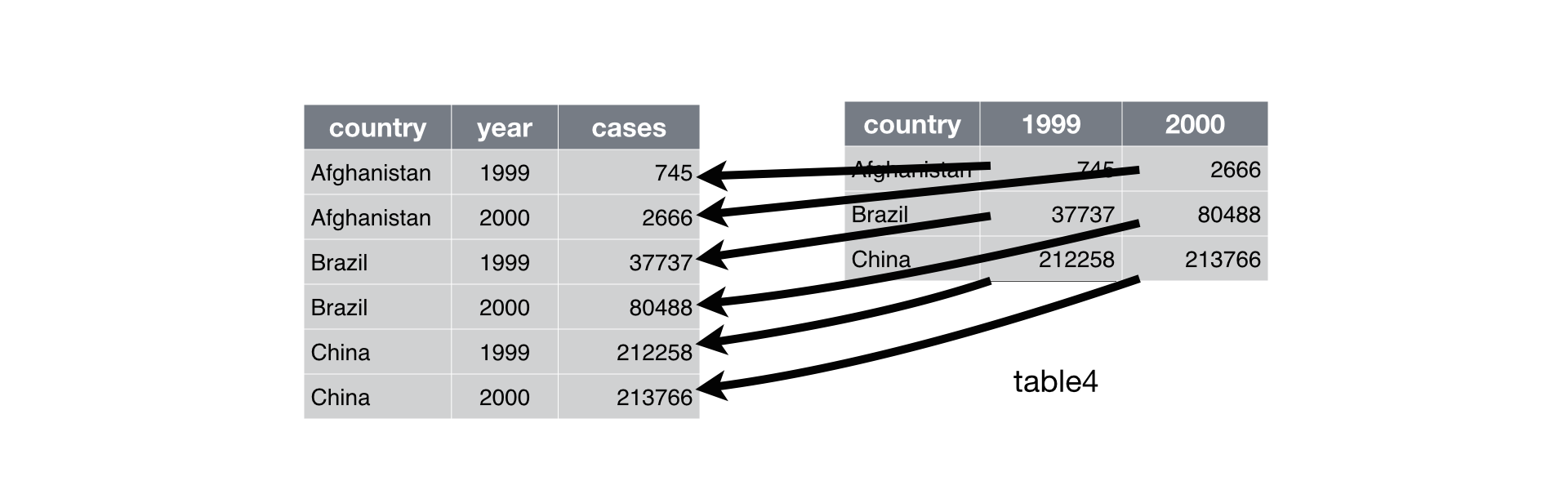
Figure 1: Convert from wide to long. Taken from R for Data Science.

To go from wide to long we use gather to sweep up a set of columns into one key-value pair. The arguments for gather are:

The name of a new column that contains the original column names
The name of a new column that contains the values from the original columns
The original columns we either want or do not want “gathered” up.

Compare how table4b looks normally and then after converting to the long form with gather().

# Original data
table4b

#> # A tibble: 3 x 3
#>   country         `1999`     `2000`
#> * <chr>            <int>      <int>
#> 1 Afghanistan   19987071   20595360
#> 2 Brazil       172006362  174504898
#> 3 China       1272915272 1280428583

# Convert to long form by stacking population by each year
# Use minue to exclude a variable (country) from being "gathered"
table4b %>% 
    gather(year, population, -country)

#> # A tibble: 6 x 3
#>   country     year  population
#>   <chr>       <chr>      <int>
#> 1 Afghanistan 1999    19987071
#> 2 Brazil      1999   172006362
#> 3 China       1999  1272915272
#> 4 Afghanistan 2000    20595360
#> 5 Brazil      2000   174504898
#> 6 China       2000  1280428583

# This does the same:
table4b %>%
    gather(year, population, `1999`, `2000`)

#> # A tibble: 6 x 3
#>   country     year  population
#>   <chr>       <chr>      <int>
#> 1 Afghanistan 1999    19987071
#> 2 Brazil      1999   172006362
#> 3 China       1999  1272915272
#> 4 Afghanistan 2000    20595360
#> 5 Brazil      2000   174504898
#> 6 China       2000  1280428583

This can be challenging to conceptually grasp at first. Let’s try an example situation when you may use gather(). Let’s say you wanted to find out the means of several characteristics of a population. You could use the group_by() and summarise() combination on their own, but another method is using gather() to group by and summarise all the variables at once.

# Keep only variables of interest
nhanes_chars <- NHANES %>% 
    select(SurveyYr, Gender, Age, Weight, Height, BMI, BPSysAve)
nhanes_chars

#> # A tibble: 10,000 x 7
#>    SurveyYr Gender   Age Weight Height   BMI BPSysAve
#>    <fct>    <fct>  <int>  <dbl>  <dbl> <dbl>    <int>
#>  1 2009_10  male      34   87.4   165.  32.2      113
#>  2 2009_10  male      34   87.4   165.  32.2      113
#>  3 2009_10  male      34   87.4   165.  32.2      113
#>  4 2009_10  male       4   17     105.  15.3       NA
#>  5 2009_10  female    49   86.7   168.  30.6      112
#>  6 2009_10  male       9   29.8   133.  16.8       86
#>  7 2009_10  male       8   35.2   131.  20.6      107
#>  8 2009_10  female    45   75.7   167.  27.2      118
#>  9 2009_10  female    45   75.7   167.  27.2      118
#> 10 2009_10  female    45   75.7   167.  27.2      118
#> # … with 9,990 more rows

# Convert to long form, excluding year and gender
nhanes_long <- nhanes_chars %>% 
    gather(Measure, Value, -SurveyYr, -Gender)
nhanes_long

#> # A tibble: 50,000 x 4
#>    SurveyYr Gender Measure Value
#>    <fct>    <fct>  <chr>   <dbl>
#>  1 2009_10  male   Age        34
#>  2 2009_10  male   Age        34
#>  3 2009_10  male   Age        34
#>  4 2009_10  male   Age         4
#>  5 2009_10  female Age        49
#>  6 2009_10  male   Age         9
#>  7 2009_10  male   Age         8
#>  8 2009_10  female Age        45
#>  9 2009_10  female Age        45
#> 10 2009_10  female Age        45
#> # … with 49,990 more rows

# Calculate mean on each measure, by gender and year
nhanes_long %>% 
    group_by(SurveyYr, Gender, Measure) %>% 
    summarise(MeanValue = mean(Value, na.rm = TRUE))

#> # A tibble: 20 x 4
#> # Groups:   SurveyYr, Gender [4]
#>    SurveyYr Gender Measure  MeanValue
#>    <fct>    <fct>  <chr>        <dbl>
#>  1 2009_10  female Age           38.0
#>  2 2009_10  female BMI           27.0
#>  3 2009_10  female BPSysAve     116. 
#>  4 2009_10  female Height       157. 
#>  5 2009_10  female Weight        67.1
#>  6 2009_10  male   Age           35.5
#>  7 2009_10  male   BMI           26.7
#>  8 2009_10  male   BPSysAve     120. 
#>  9 2009_10  male   Height       168. 
#> 10 2009_10  male   Weight        76.3
#> 11 2011_12  female Age           37.3
#> 12 2011_12  female BMI           26.5
#> 13 2011_12  female BPSysAve     117. 
#> 14 2011_12  female Height       156. 
#> 15 2011_12  female Weight        65.3
#> 16 2011_12  male   Age           36.2
#> 17 2011_12  male   BMI           26.4
#> 18 2011_12  male   BPSysAve     120. 
#> 19 2011_12  male   Height       167. 
#> 20 2011_12  male   Weight        75.3

Note that summarising by mean can only be done with continuous variables. Anyway, with the long form, you can do more with less code ☺️

`spread()`: (If time) Converting from long to wide form

You can also convert to wide from long. This is not as commonly done, since most analyses are better in the long form. But sometimes you may need to have a wide form. Here you can use spread(), which takes three arguments: 1) the data, 2) the key column (or column with identifying information), 3) the value column (the one with the numbers/values). We’ll use a pipe so we can ignore the data argument.

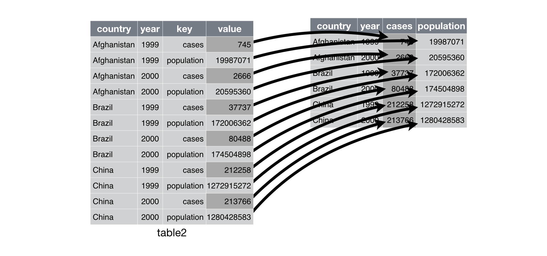
Figure 2: ‘Spreading’ from long to wide. Taken from the R for Data Science book.

# Using a small dataset:
table2

#> # A tibble: 12 x 4
#>    country      year type            count
#>    <chr>       <int> <chr>           <int>
#>  1 Afghanistan  1999 cases             745
#>  2 Afghanistan  1999 population   19987071
#>  3 Afghanistan  2000 cases            2666
#>  4 Afghanistan  2000 population   20595360
#>  5 Brazil       1999 cases           37737
#>  6 Brazil       1999 population  172006362
#>  7 Brazil       2000 cases           80488
#>  8 Brazil       2000 population  174504898
#>  9 China        1999 cases          212258
#> 10 China        1999 population 1272915272
#> 11 China        2000 cases          213766
#> 12 China        2000 population 1280428583

# Convert to wide form
table2 %>% 
    spread(key = type, value = count)

#> # A tibble: 6 x 4
#>   country      year  cases population
#>   <chr>       <int>  <int>      <int>
#> 1 Afghanistan  1999    745   19987071
#> 2 Afghanistan  2000   2666   20595360
#> 3 Brazil       1999  37737  172006362
#> 4 Brazil       2000  80488  174504898
#> 5 China        1999 212258 1272915272
#> 6 China        2000 213766 1280428583

The key is the discrete value that will make up the new column names, while the value will be column that will make up the values of the new columns.

Final exercise: Replicate the output from the given dataset.

Time: Until end of the session.

In the exercise-wrangling.R file, copy the code below to get the data into the form needed. Using everything you learned in this session, try to recreate the table below from the dataset given here.

NHANES

#> # A tibble: 10,000 x 76
#>       ID SurveyYr Gender   Age AgeDecade AgeMonths Race1 Race3 Education
#>    <int> <fct>    <fct>  <int> <fct>         <int> <fct> <fct> <fct>    
#>  1 51624 2009_10  male      34 " 30-39"        409 White <NA>  High Sch…
#>  2 51624 2009_10  male      34 " 30-39"        409 White <NA>  High Sch…
#>  3 51624 2009_10  male      34 " 30-39"        409 White <NA>  High Sch…
#>  4 51625 2009_10  male       4 " 0-9"           49 Other <NA>  <NA>     
#>  5 51630 2009_10  female    49 " 40-49"        596 White <NA>  Some Col…
#>  6 51638 2009_10  male       9 " 0-9"          115 White <NA>  <NA>     
#>  7 51646 2009_10  male       8 " 0-9"          101 White <NA>  <NA>     
#>  8 51647 2009_10  female    45 " 40-49"        541 White <NA>  College …
#>  9 51647 2009_10  female    45 " 40-49"        541 White <NA>  College …
#> 10 51647 2009_10  female    45 " 40-49"        541 White <NA>  College …
#> # … with 9,990 more rows, and 67 more variables: MaritalStatus <fct>,
#> #   HHIncome <fct>, HHIncomeMid <int>, Poverty <dbl>, HomeRooms <int>,
#> #   HomeOwn <fct>, Work <fct>, Weight <dbl>, Length <dbl>, HeadCirc <dbl>,
#> #   Height <dbl>, BMI <dbl>, BMICatUnder20yrs <fct>, BMI_WHO <fct>,
#> #   Pulse <int>, BPSysAve <int>, BPDiaAve <int>, BPSys1 <int>,
#> #   BPDia1 <int>, BPSys2 <int>, BPDia2 <int>, BPSys3 <int>, BPDia3 <int>,
#> #   Testosterone <dbl>, DirectChol <dbl>, TotChol <dbl>, UrineVol1 <int>,
#> #   UrineFlow1 <dbl>, UrineVol2 <int>, UrineFlow2 <dbl>, Diabetes <fct>,
#> #   DiabetesAge <int>, HealthGen <fct>, DaysPhysHlthBad <int>,
#> #   DaysMentHlthBad <int>, LittleInterest <fct>, Depressed <fct>,
#> #   nPregnancies <int>, nBabies <int>, Age1stBaby <int>,
#> #   SleepHrsNight <int>, SleepTrouble <fct>, PhysActive <fct>,
#> #   PhysActiveDays <int>, TVHrsDay <fct>, CompHrsDay <fct>,
#> #   TVHrsDayChild <int>, CompHrsDayChild <int>, Alcohol12PlusYr <fct>,
#> #   AlcoholDay <int>, AlcoholYear <int>, SmokeNow <fct>, Smoke100 <fct>,
#> #   Smoke100n <fct>, SmokeAge <int>, Marijuana <fct>, AgeFirstMarij <int>,
#> #   RegularMarij <fct>, AgeRegMarij <int>, HardDrugs <fct>, SexEver <fct>,
#> #   SexAge <int>, SexNumPartnLife <int>, SexNumPartYear <int>,
#> #   SameSex <fct>, SexOrientation <fct>, PregnantNow <fct>

Table 1: Mean values of characteristics for women and men between 18-75 years of age at each of the two survey years.
Gender	Measure	2009_10	2011_12
female	Age	44.02	44.15
female	AgeDiabetesDiagnosis	48.13	46.51
female	BMI	28.96	28.60
female	BPDiaAve	67.69	70.04
female	BPSysAve	116.04	117.90
female	DrinksOfAlcoholInDay	2.34	2.20
female	MoreThan5DaysActive	0.31	0.39
female	NumberOfBabies	2.44	2.31
female	Poverty	2.93	2.88
female	TotalCholesterol	5.14	5.11
male	Age	43.11	43.88
male	AgeDiabetesDiagnosis	47.58	45.14
male	BMI	28.76	28.70
male	BPDiaAve	70.94	73.14
male	BPSysAve	121.61	122.43
male	DrinksOfAlcoholInDay	3.52	3.71
male	MoreThan5DaysActive	0.29	0.36
male	NumberOfBabies	NaN	NaN
male	Poverty	3.01	2.97
male	TotalCholesterol	5.07	4.90

Resources for learning and help

For learning:

“R for Data Science” book: Tidy Data chapter
tidyr vignette
dplyr vignette

For help:

Data wrangling cheatsheet
StackOverflow for tidyr
StackOverflow for dplyr
Quick package information using RStudio: ?tidyr, ?dplyr

Acknowledgements

Parts of this lesson were modified from a session taught at the Aarhus University Open Coders, with contributions from Elena Dudukina, PhD student at AU in Clinical Epidemiology, as well as from the dplyr sessions of the UofTCoders course. Much inspiration was also taken from the R for Data Science book.

Last updated on Mar 4, 2019

Data management, wrangling, and best practices

Session details

Objectives

Expected learning

Managing and working with data in R

Loading the packages and dataset

Exercise: Become familiar with the dataset

“Messy” vs. “tidy” data

%>%: The pipe operator

mutate(): Transforming or adding variables

Exercise: Piping, transforming, and adding

select(): Select specific data by the variables

rename(): Rename specific columns

filter(): Filtering/subsetting the data by row

arrange(): Sorting/(re)arranging your data by column

Exercise: Filtering and logic, arranging, and selecting

group_by(), summarise(): Create a summary of the data, alone or by a group(s)

gather(): Converting from wide to long form

spread(): (If time) Converting from long to wide form

Final exercise: Replicate the output from the given dataset.

Resources for learning and help

Acknowledgements

`%>%`: The pipe operator

`mutate()`: Transforming or adding variables

`select()`: Select specific data by the variables

`rename()`: Rename specific columns

`filter()`: Filtering/subsetting the data by row

`arrange()`: Sorting/(re)arranging your data by column

`group_by()`, `summarise()`: Create a summary of the data, alone or by a group(s)

`gather()`: Converting from wide to long form

`spread()`: (If time) Converting from long to wide form